About Interpolation 補間について

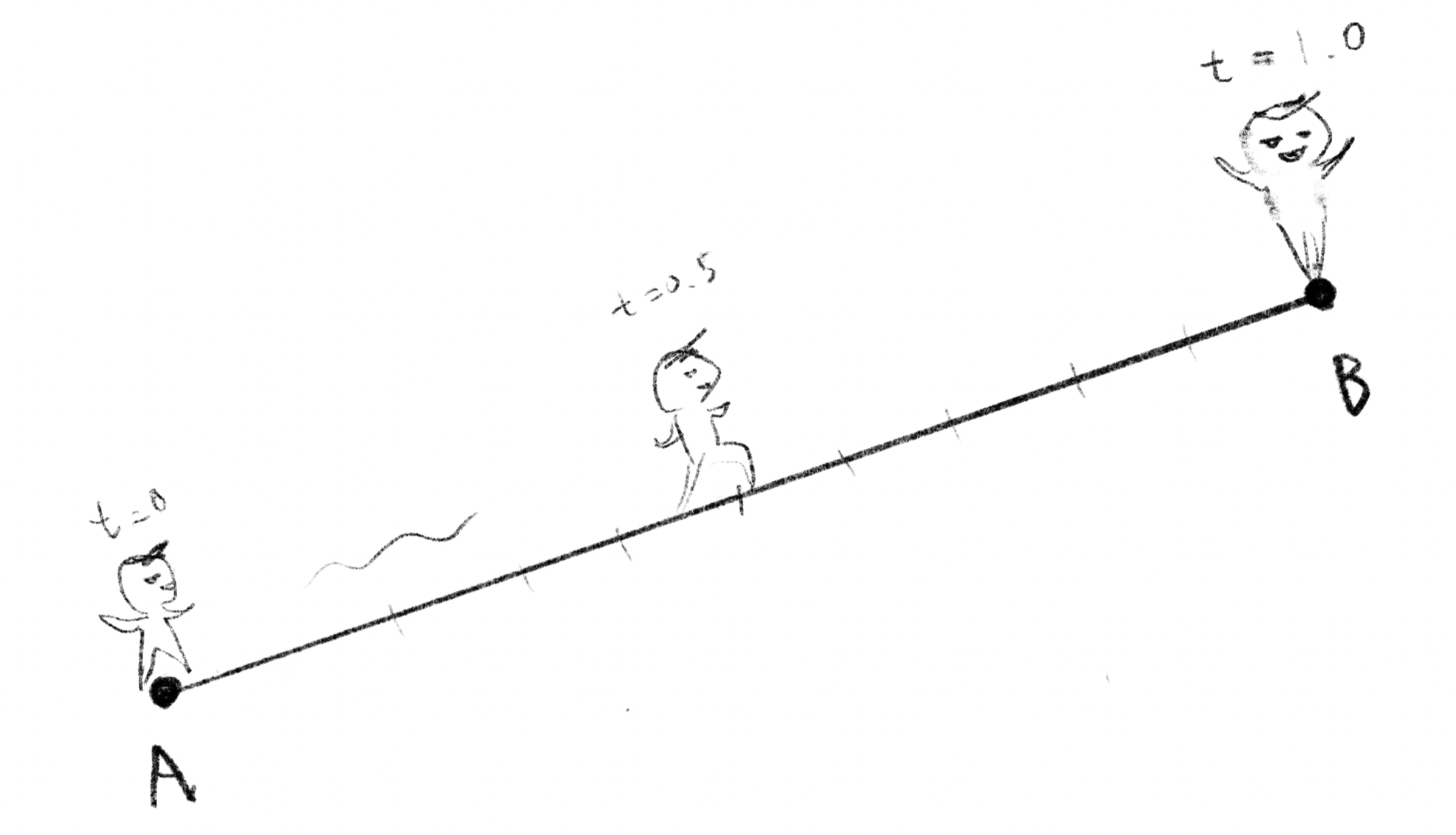
Interpolation is about estimating the values that lie between the points you already know. When you’re moving a character from point A to B, you interpolate between them so you know where the character is at a given time. You know the stock price in May and July, so you interpolate between them to estimate what the price was in June. The idea is so simple, and applicable to so many things.

補間とは、すでに知っている点と点の間の値を推測することです。たとえば、キャラクターがA地点からB地点まで移動する場合に、ある時点でキャラクターがどこにいるかを知るために補間を使います。5月と7月の株価が分かれば、その間を補間して6月の株価を推定できます。このシンプルなアイデアは、様々な場面で使えます。

This is an article to introduce various topics in Sketching with Code, illustrating the relationships between them and adding more context to provide a sort of overview. The articles are not in order of difficulty. Please just jump to whichever one interests you.

これは Sketching with Math and Quasi Physics 上の様々なトピックについて、それぞれの間の関係や概要を示したり、新たな文脈を加えたりするためのページです。難易度順には並んでいないので、興味のある記事から自由に読んでみてください。

Linear Interpolation

線形補間

Let’s start from the simplest case where the value changes at the same rate all the way.

最もシンプルな、値が一定の割合で変化する場合から始めましょう。

Suppose that point $P$ moves from one point $A$ to another point $B$, and the variable $t$ is the ratio how much $P$ has moved between them. If $t = 0$, $P$ is in the same position as $A$. If $t = 1$, $P$ is in the same position as $B$, and if $t = 0.5$, $P$ is exactly at the midpoint between $A$ and $B$. This can be expressed as follows. $A$, $B$, and $P$ can be either numbers or vectors.

ある点$A$から別の点$B$まで点$P$が移動するとします。$P$の移動した割合を$t$という変数で表します。$t = 0$ なら$P$は$A$と同じ位置、$t = 1$ なら$P$は$B$と同じ位置、$t=0.5$ なら$P$はちょうど$A$と$B$の中点にいるという具合です。これは下記のように表せます。$A$, $B$, $P$ は数値でもベクトルでも構いません。

$P = (1 - t)\cdot A + t \cdot B$

If we interpolate between points in 2D, we can draw a line segment.

2次元上の点と点の間を補間すれば、線分が描けます。

$x(t) = (1-t)x_1 + tx_2$
$y(t) = (1-t)y_1 + ty_2$

Easing functions

イージング関数

But things don’t always change at the same pace. To manipulate the rate, we use different functions called easing functions. Easing functions are not a clearly defined category, and they can be any function that can map a range of values (usually 0 to 1) to the same range continuously, keeping the start and end the same.

しかし、物事はいつも一定の割合で変化するわけではありません。変化の様子をコントロールするために、イージング関数と呼ばれる様々な関数が使えます。イージング関数はきちんと定義されたカテゴリーではなく、ある値の範囲（通常は0から1）を同じ範囲に連続的に写像し、始点と終点を保持できる関数ならなんでも使えます。

Mapping 写像

Bézier and Spline

ベジェとスプライン

On a one dimensional line, you can draw only a single path between two points, but in higher dimensions, like 2D or 3D, there are infinite ways to connect two dots. Defining a path between points in flexible but precise way is very crucial for computer graphics to draw lines and shapes.

1次元の直線上では2点の間を結ぶ経路は1つだけですが、2次元や3次元のような高次元では、2点を結ぶ方法は無限にあります。コンピューターグラフィックスで線や形を描くためには、点と点の間の経路を柔軟かつ正確に定義することが不可欠です。

One of the most common methods called Bézier curve is basically to repeat linear interpolations multiple times. The demo below illustrates this idea.

ベジェ曲線は、最も一般的な手法の1つで、線形補間を複数回繰り返すことで作られます。下のデモでこの考え方を見ることができます。

Bézier and Spline ベジェとスプライン

There are many different methods to draw curved lines similar to Bézier curves but with more advanced features. For example, B-spline introduces additional parameters to adjust the weights of each point to add more nuanced control over the line’s shape.

ベジェ曲線に似た曲線を描く手法には、より高度な機能を持つものが色々あります。例えばBスプラインは各点に重みを設定するパラメータを追加することで、曲線の形状をより精密にコントロールできます。

Smoothness and Continuity

なめらかさと連続性

When we draw curves, we often care how smooth they are. What smooth means can vary, but to deal with a specific kind of smoothness, there is a very useful mathematical concept called continuity.

曲線を描くときには、その滑らかさが気になります。滑らかさという言葉の意味は場合によりますが、ある特定の種類の滑らかさを扱うために、連続性というとても便利な数学の概念があります。

To measure how smooth a curve is in a mathematical sense, you can take the derivative of the function that represents the curve. The first derivative shows the rate of change of position, and the second derivative shows the rate of change of the rate of change.

曲線の滑らかさを数学的に測るには、その曲線を表す関数の微分を取ることができます。最初の微分は位置の変化率を示し、2度目の微分はその変化率の変化を示します。このようにすると、異なるレベルの連続性を考えることができます。

• $C^0$ Continuity: The curve itself is continuous. There are no breaks or gaps. You can imagine a line without lifting your pen. There is no gap in this line, but there can be sharp corners and turns that may not appear smooth.

• $C^1$ Continuity: The first derivative of the curve is continuous. This means the curve has no sharp corners or cusps; it changes direction smoothly. You can think of a smoothly curving road without any sudden turns.

• $C^2$ Continuity: The second derivative of the curve is continuous. This means that even the rate at which the curve changes direction is continuous. Roller coasters are usually designed to have $C^2$ continuity as much as possible to avoid too sudden a change in acceleration, which can be uncomfortable or even harmful to the passengers. If it is not $C^2$ continuous, sudden changes in G-forces might slam you into the seat or cause whiplash.

• $C^0$連続: 曲線に途切れや隙間がなく連続しています。ペンを持ち上げずに描いた線を想像してください。この線には途切れた箇所はありませんが、滑らかに見えない鋭い角や曲がった部分があるかもしれません。

• $C^1$ 連続: 曲線の1次微分が連続です。これは、曲線が滑らかに方向を変え鋭い角や尖った点がないことを意味します。突然の折れ曲りがない滑らかな道路を想像してみましょう。

• $C^2$ 連続: 曲線の2次微分が連続です。これは、曲線が向きを変える速ささえも滑らかであることを意味します。ジェットコースターは、乗客に不快さや危険を与えないよう、できるだけ$C^2$連続性を持つように設計されています。$C^2$連続でない場合、急なGの変化で体を席に打ちつけたり、むち打ち症になったりするかもしれません。

An algorithm called natural spline is designed to guarantee $C^2$ Continuity at any point along a curve that passes through multiple points.

ナチュラルスプラインと呼ばれるアルゴリズムは、複数の点を通る曲線のどの位置においても$C^2$連続性を保証するように設計されています。

While a natural spline is mathematically smooth, it may not always look like the smoothest line to human eyes. The Hobby curve algorithm minimizes curvature at each point along the line, making strokes that look like Henri Matisse’s stroke drawn with a very long brush.

ナチュラルスプラインは数学的には滑らかですが、人間の目には必ずしも最も滑らかな線には見えないかもしれません。Hobby曲線というアルゴリズムは線上のそれぞれ点での曲率を最小限に抑え、アンリ・マティスが長い筆で描いたようなストロークを描くことができます。

Controlling curves 曲線のコントロール

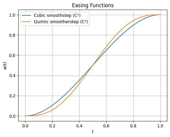
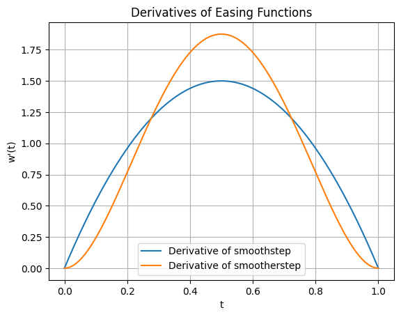
Smoothstep functions

スムースステップ関数

For connecting lines or interpolations smoothly, Hermite interpolation, or so-called smoothstep functions are often used. When $t$ moves from 0 to 1, these functions can adjust the rate of change to make the derivative at the beginning and the end be zero. The first formula guarantees $C^1$ continuity and the second one is for $C^2$, the last one is the general form for any level of continuity. The formulas themselves are not very intuitive, but if you look at the graphs below, you can visually confirm that the rate of change becomes zero. The graph to the left shows the first derivative, and the one to the right shows the second derivative.

線や補間を滑らかにつなぐには、エルミート補間（スムースステップ関数とも呼ばれる）がよく使われます。この関数は$t$が0から1に移動する際の変化率を調整して、始点と終点での微分値をゼロにすることができます。最初の式は$C^1$連続性を保証し、2番目の式は$C^2$用、最後の式はあらゆる連続性レベルに対応する一般形です。式自体は直感的ではありませんが、下のグラフを見れば変化率がゼロになることが視覚的に分かります。左のグラフは1次微分を、右のグラフは2次微分を表しています。

$w_{C^{1}}(t)\;=\;3\,t^{2}-2\,t^{3}$

$w_{C^{2}}(t)\;=\;6\,t^{5}-15\,t^{4}+10\,t^{3}$

$\begin{aligned} w_{C^{n}}(t)\;=\; \sum_{k=0}^{n} (-1)^{k}\, \binom{n+k}{\;k}\, \binom{2n+1}{\,n-k}\; t^{\,n+1+k} \end{aligned}$

Google Colab

https://colab.research.google.com/drive/1wW3HOI6GRnORn7qUCH150HNbi9FFD-ZS#scrollTo=8klcv3tWGVVb

For example, these demos for the noise functions from the Taming Randomness ランダムさを手なづける page use the Hermite functions.

例えば、Taming Randomness ランダムさを手なづけるページのノイズ関数のデモでエルミート関数が使われています。

Interpolation for many arbitrary points

たくさんの点についての補間

Instead of trying to control the interpolation precisely, there are methods to use algorithms to figure out the exact way to interpolate between points. This is particularly useful when there are multiple data points spread across a space.

補間を完全にコントロールするのではなく、アルゴリズムを使って点と点の間を自動的に補間する手法もあります。この方法は、特に空間上に多くのデータポイントが散らばっている場合に効果的です。

RBF interpolation is one of those methods. It solves for weights automatically and produces a smooth surface that passes through however many points you throw at it, even in higher dimensions.

RBF補間はそのような手法の1つです。重みを自動的に算出し、何次元の空間でも、与えられた点の数に関わらず、すべての点を通る滑らかな曲面を作り出します。

Take a look at the demo of RBF interpolation in 2D space. You can drag white points to play around.

2次元空間でのRBF補間のデモを見てみましょう。白い点をドラッグしてみてください。

Continuous Mapping 連続的な写像

Mixing Colors

色を混ぜる

Interpolation is not just about moving things and drawing lines. Colors are another good example. You can mix two or more colors by interpolating between them. Your result can be different depending on which color model you use. You could even draw a curved line in a color space to get an interesting gradient.

補間は、物を動かしたり線を引いたりするだけではありません。色も良い例です。2つ以上の色を補間すると色を混ぜることができます。どの色空間モデルを使うかによって結果は異なります。色空間の中で曲線を描くことで、面白いグラデーションを作ることもできます。

You might have seen a menu to select (re)sampling method when you are resizing an image in graphics software like Adobe Photoshop. These software programs take colors from the closest pixels and interpolate between them. In case of Photoshop, “Nearest Neighbor” means no interpolation (just pick a color from a single closest pixel), “Bilinear” linearly blends the 2 × 2 neighborhood, “Bicubic” uses a cubic function to give it $C^1$ continuity.

Adobe Photoshopなどのグラフィックソフトウェアで画像サイズを変更する時に、サンプリング方式を選ぶメニューを見たことがあるかもしれません。これらのソフトウェアは、近くのピクセルから色を拾って、それらの間を補間します。Photoshopの場合、「ニアレストネイバー」は補間を行わず（単純に最も近いピクセルの色を使う）、「バイリニア」は2×2の近傍を線形的にブレンドし、「バイキュービック」は三次関数を使用して$C^1$連続性を実現します。

Mixing Colors 色を混ぜる

Interpolating everything

なんでも補間する

As you might have noticed already at this point, you can interpolate between anything that can be represented as vectors. By seeing things through the lens of concepts like vectors and interpolation, we can treat many things in the same way (that is the power of abstraction). Interpolation is indeed a powerful and versatile technique to add to your toolbox.

もう気づいていると思いますが、ベクトルとして表現できるものは何でも補間することができます。ベクトルや補間といった概念を通して物事を見ることで、多くのものを同じ方法で扱うことができます。（これが抽象化の力です）補間は道具箱に入れておくべき、強力で汎用性の高いテクニックです。

There is a very similar and related concept called extrapolation. As the name suggests, extrapolation is to extend a line beyond the ends. Extrapolation is used to predict values beyond the boundary of known data points (predict the future!). It’d be interesting to explore this topic too if you are interested.

外挿（extrapolation）という、よく似た、関連のある概念があります。名前が示す通り、外挿とは線を端点の先まで延長することです。外挿は、既知のデータポイントの境界を超えた値を予測する（例えば未来を予測する）ために使用されます。興味があれば外挿についても調べてみると良いでしょう。