Bézier and Spline ベジェとスプライン

A spline is a curve mathematically defined by a series of control points.

スプラインは、一連の制御点によって数学的に定義された曲線です。

We learned about different curves that can be defined with the parametric approach on the previous page. The problem is that they require different formulas for each shape. To draw various shapes more freely, we need a more flexible method.

前のページではパラメトリックなアプローチで定義できるさまざまな曲線について学びましたが、問題は、形ごとに異なる公式が必要になってしまうことです。様々な形をより自由に描くには、より柔軟な手法が必要です。

Spline curve

スプライン曲線

A spline curve is a mathematically defined curve that smoothly passes through or is close to a series of control points. It is like a big family, and there are many variations including Bézier curves, B-spline curves, NURBS (Non-Uniform Rational B-Splines), Cardinal Splines, Catmull-Rom Splines, Hermite Splines, etc.

スプライン曲線は、滑らかに一連の制御点を通過するか、またはその近くを通過するように数学的に定義された曲線です。これは大きなファミリーのようなもので、例えば、ベジェ曲線、Bスプライン曲線、NURBS（Non-Uniform Rational B-Splines）、カーディナルスプライン、Catmull-Rom スプライン、エルミートスプラインなどに様々なバリエーションがあります。

The term “spline” comes from the fact that draftsmen used flexible strips of metal or wood to draw smooth curves between points. But today, it typically refers to curves defined by polynomial functions instead of physical pieces. From this family, we will examine the Bezier curve and its expansion, B-Spline.

「スプライン」という言葉は、製図に使われていた、点と点の間に滑らかな曲線を描くための金属や木の柔軟な帯に由来します。しかし、今日では、通常、物理的な部品ではなく多項関数によって定義された曲線を指します。この家族から、ベジエ曲線とその拡張であるBスプラインを検討します。

Bézier curve

ベジェ曲線

See also the Interpolation and Animation page.
補間とアニメーションのページもご覧ください。

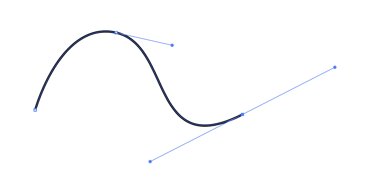
Bezier curves, especially cubic Bézier curves, are widely used for drawing shapes in computer software, probably because they can be intuitively visualized with control points and “handles,” which are suitable for manipulation with a GUI. For example, the image below is a screenshot from Adobe Illustrator.

ベジェ曲線、特に3次ベジェ曲線は、ソフトウェアで図形を描くために幅広く使われています。制御点と「ハンドル」を使って直感的に操作できるため、GUIでの操作にも適しています。下の画像はAdobe Illustratorのスクリーンショットの例です。

Interpolating Interpolations

補間の補間

The basic idea of a Bézier curve is to repeat linear interpolations multiple times. Remember the parametric line segment from the previous page.

ベジェ曲線の基本的なアイデアは、線形補間を複数回繰り返すことです。前のページで触れた線分のパラメトリックな表現を思い出してください。

$x(t) = (1-t)x_1 + tx_2$
$y(t) = (1-t)y_1 + ty_2$

Though this is not curved at all, this is called a Bézier curve of degree 1, or a linear Bézier curve.

全く曲がってはいませんが、これを1次のベジェ曲線、または線形ベジェ曲線と呼びます。

Now we can combine two line segments defined by three points to draw a line that actually curves.

ここで、3つの点で定義された2つの線分を組み合わせると、実際に曲線を描くことができます。

Say there are three points, $p_1$, $p_2$, $p_3$. We interpolate between $p_1$ and $p_2$, and $p_2$ and $p_3$, then interpolate between two resulting points. this is called a Bézier curve of degree 2, or a quadratic Bézier curve.

3つの点、$p_1$、$p_2$、$p_3$があるとします。$p_1$ と $p_2$ の間、 $p_2$ と $p_3$ の間を補間し、さらにこの補間の結果得られた2つの点の間を補間します。これを2次ベジェ曲線と呼びます。

You can use as many points as you want. These are referred to as quadratic Bezier curves (3 points), cubic Bezier curves (4 points), quartic Bezier curves (5 points), etc., or a Bezier curve of degree N (where N is the number of points minus one). The cubic version is most commonly used. In the demo below, you can drag and move the points to draw different curves.

点の数はいくら増やしても構いません。これらは2次ベジェ曲線（3点）、3次ベジェ曲線（4点）、4次ベジェ曲線（5点）といったようにN次ベジェ曲線（Nは点の数から1を引いた値）と呼ばれますが、3次のベジェ曲線が最も一般的に使用されます。下のデモでは、点をドラッグして移動し、様々な曲線を描くことができます。

Notice that the computeBezierPoint is a recursive function that can take any number of points. Try drawing the Bézier curves of different degrees and how the positions of points affects the shape.

computeBezierPoint は任意の数の点を引数に取る再帰関数であることに注目してください。様々な次数のベジェ曲線を描いて、点の位置が形状にどのように影響するかを試してみてください。

computeBezierPoint(points, t, debugDraw) {
    let n = points.length;
    if (n === 1) {
      return points[0];
    }
    let newPoints = [];
    for (let i = 0; i < n - 1; i++) {
      const pa = points[i];
      const pb = points[i + 1];
      const pc = createVector(lerp(pa.x, pb.x, t), lerp(pa.y, pb.y, t));
      newPoints.push(pc);
      
      if (debugDraw) {
        stroke(0, 0, 0, 32);
        line(pa.x, pa.y, pb.x, pb.y);
        fill(0);
        circle(pc.x, pc.y, 6);
      }
    }
    return this.computeBezierPoint(newPoints, t, debugDraw);
  }

Bernstein Polynomial

バーンスタイン多項式

Repeating linear interpolations is a flexible and intuitive way, but is not very computationally efficient. In practical implementations, we often use the form called Bernstein Polynomial. The below is the Bernstein polynomial for cubic Bézier.

線形補間を繰り返す方法は柔軟で直感的ですが、計算効率はあまり良くありません。実用向けの実装では、バーンスタイン多項式と呼ばれる形が良く使われます。以下は、3次ベジェ曲線のバーンスタイン多項式です。

$B(t) = (1 - t)^3 P_0 + 3(1 - t)^2 t P_1 + 3(1 - t) t^2 P_2 + t^3 P_3$

This form can be derived from the linear version with a bit of calculation.

この形は、少し計算することで線形のバージョンから導き出すことができます。

We start from the “linear interpolation of linear interpolations”

「線形補間の線形補間」からスタートします。

$Q_0(t) = (1 - t)P_0 + tP_1$

$Q_1(t) = (1 - t)P_1 + tP_2$

$B(t) = (1 - t)Q_0(t) + tQ_1(t)$

If you substitute $Q_0(t)$ and $Q_1(t)$ into the last line:

最後の行の $Q_0(t)$ と $Q_1(t)$ を置き換えると下記のようになります。

$B(t) = (1 - t)[(1 - t)P_0 + tP_1] + t[(1 - t)P_1 + tP_2]$

Then you can expand and combine like terms to get the Bernstein version.

次に、展開して同類項を結合すると、バーンスタイン版の式が得られます。

$B(t) = (1 - t)^3 P_0 + 3(1 - t)^2 t P_1 + 3(1 - t) t^2 P_2 + t^3 P_3$

If you look closely at this formula, you can see it as a weighted average of the four control points, where the weights of the points change as $t$ moves from 0. When $t = 0$, $P_0$ has 100% of the weight. Then, other points start to gain more weight as $t$ increases. At the end ($t = 1$), $P_3$ will have 100% of the weight.

よく見ると、この式は4つの制御点の重み付き平均として解釈できます。点の重みは $t$ が 0 から動くにつれて変化します。$t = 0$ のとき、$P_0$ は100%の重みを持ちます。その後、$t$ が増加するにつれて重みが他の点に移動しま始めます。最終的に ($t = 1$ のとき)、$P_3$ の重みが100%になります。

The demo below uses a class Cubic that implements the Bernstein Polynomial for cubic Bézier.

下のデモでは、3次ベジェのバーンスタイン多項式を実装した Cubic クラスを使っています。

getPointAt(t) {
      const u = 1 - t;
      return new p5.Vector(
          this.a0.x * (u * u * u) + this.c0.x * (3 * t * u * u) +
          this.c1.x * (3 * t * t * u) + this.a1.x * (t * t * t),
          this.a0.y * (u * u * u) + this.c0.y * (3 * t * u * u) +
          this.c1.y * (3 * t * t * u) + this.a1.y * (t * t * t)
      );
  }

Even better, p5.js has a function bezier() specifically for drawing a cubic Bézier curve. The draw() function of the Cubic class can be replaced with this function.
さらに簡単なことに、p5.jsには3次ベジェ曲線を描画するための bezier() という関数があります。Cubic クラスの draw() 関数はこの関数で置き換えることができます。

Higher-order Bézier Curve

高次ベジェ曲線

As mentioned earlier, you can use any number of points to define a Bézier curve. Though it may not be practically useful, Bézier curves of higher degree are fun to look at. Take a look at the demo below.

先に触れた通り、ベジェ曲線は任意の数の点を使って定義できます。あまり実用的ではありませんが、高次のベジェ曲線はなかなか楽しい見た目になります。下のデモを見てみましょう。

B-Spline

Bスプライン

Bézier curves are great for drawing flexible curves, but some people wanted even more precise control over the shape.

ベジェ曲線は柔軟に描くためにとても便利ですが、さらに正確に形を制御したいと思う人もいます。

B (Basis)-Spline is one of those methods and is an expansion or generalization of the Bézier curve. The Bézier curves have constraint that you can’t adjust how each control point affects the shape because the influence is fixed. B-splines introduce knot vector, which are numbers that control the influence or weights of the control points along the curve, giving you more control over the shape.

B（ベース）スプラインは、そのための手法の1つ、ベジェ曲線の拡張または一般化です。ベジェ曲線にはそれぞれの制御点が形状に与える影響が固定されていて、調整できないという制限があります。Bスプラインはノットベクターという、曲線に沿った制御点の影響、または重みをコントロールするため数値を取り入れることで、より自由な形の制御を可能にします。

B-splines have three elements to define a curve.

Bスプラインには、曲線を定義するための3つの要素があります。

• Control Points: Control points act like centers of gravity that pull the curve towards them. Their influence changes as the parameter $t$ changes, moving the point along a curved line. You can use any number of control points.

• Degree (d) : This defines the degree of the polynomial segments that make up the B-spline. For example, a degree of 3 means cubic polynomial segments. This means that (d + 1) control points will influence each segment of the curve.

• Knot vector: This is a sequence of parameter values that determine where and how the control points affect the B-spline curve. They divide the parameter into intervals and influence the blending of the polynomial segments.

• 制御点：制御点は、曲線をそれぞれに向かって引っ張る重心のように働きます。制御点の影響はパラメータ $t$ が変化するにつれて変わり、それによって点が曲線に沿って移動します。制御点はいくつあっても構いません。

• 次数 (d) : Bスプラインを構成する、多項式によって表されたセグメントの次数です。例えば、次数が3の場合、セグメントは3次多項式で表されます。それぞれの曲線セグメントに(d + 1)個の制御点が影響を与えることになります。

• ノットベクトル: これは、制御点がBスプライン曲線にどのように影響を与えるかを決定するパラメータ値の数列です。ノットベクトルは、パラメータを区間に分割し、多項式セグメントの間の移り変わりに影響を与えます。

How all these work together? Let’s look at a demo before diving into the math. You can click on the canvas to get a random new curve.

これらはどのように連携するのでしょう。数式の前にデモを見てみましょう。キャンバスをクリックすると、ランダムな新しい曲線を表示できます。

Can you see that the weights of the control points change over time, or as $t$ increases? In the graph at the bottom, the horizontal axis is $t$, and the vertical axis is the weight of each point.

制御点の重みが時間とともに、または $t$ が増加するにつれて変化するのがわかるでしょうか。下側にあるグラフでは、横軸が $t$ 、縦軸が各点の重みを表しています。

To get the weights of the points, you start from something called basis function $N_{i,d}(t)$.

点の重みを計算するには、基底（basis）関数と呼ばれる関数 $N_{i,d}(t)$ から始めます。

Here, $i$ is the index of the control point, $d$ is the degree, and $t$ is the parameter. $u$ is an array of the knots. In the initial state of the demo above, the knots are $(0,0,1,1,2,2,3,3,4,4,5,5)$.

ここで、$i$ は制御点のインデックス、$d$ は次数、$t$ はパラメータを表します。$u$ はノットの配列です。上記のデモの初期状態では、ノットは $(0,0,1,1,2,2,3,3,4,4,5,5)$ です。

If the degree is zero:

次数がゼロの場合

$N_{i,0}(t) = \begin{cases} 1 & \text{if } u_i \leq t < u_{i+1} \ 0 & \text{otherwise} \end{cases}$

If the degree is more than zero:

次数がゼロ以上の場合

${\begin{aligned} N_{i,d}(t) = \frac{t - u_i}{u_{i+d} - u_i} N_{i,d-1}(t) + \frac{u_{i+d+1} - t}{u_{i+d+1} - u_{i+1}} N_{i+1,d-1}(t) \end{aligned}}$

This formula is recursive. Notice that $N_{i,d-1}(t)$ and $N_{i+1,d-1}(t)$ are multiplied to the left and right terms. The calculation continues until reaching the case where $d = 0$, and along the way, you compute the weights over $d+1$ knots. This is not a very easy function to grasp by just looking at it. Try substituting the variables with concrete values to get a sense of how this works.

この式は再帰的です。$N_{i,d-1}(t)$ と $N_{i+1,d-1}(t)$ が左と右の項に掛けられていることに注意してください。計算は $d = 0$ の場合に達するまで続き、その過程で $d+1$ 個のノットを計算に入れて重みを求めます。見ただけではわかりにくいので、具体的な値を変数を代入して、この仕組みがどのように働くのか試してみましょう。

Once you have the $N_{i,d}(t)$ values for all the control points, you can use them to get the weighted sum.

すべての制御点の $N_{i,d}(t)$ の値が得られたら、重み付き合計が計算できます。

$P(t) = \sum_{i=0}^{n} N_{i,d}(t) \mathbf{P}_i$

Try experimenting in the demo by changing the number of control points (numPoints), degree (degree), and knots (knots). Note that you need (numPoints + degree + 1) knots, and each knot value must be equal to or larger than the previous one.

デモ上で、制御点の数（numPoints）、次数（degree）、ノット（knots）を変えて実験してみましょう。ノットの数は（numPoints + degree + 1）必要であり、それぞれのノットの値はその前の値以上でなければならないことに注意してください。

Other mathematically defined curves

その他の数式による曲線

As we touched upon in the beginning, there are many more methods for defining curves. For example, NURB (Non-Uniform Rational B-Splines) is a further expansion of B-Spline curve, which can represent a wider variety of shapes, including exact representations of standard geometric forms like circles and ellipses. Because of the flexibility and accuracy, NURB is used as a standard representation of curves in most of CAD (Computer-Aided Design) software for product design, architecture, hardware engineering, etc.

冒頭で触れたように、曲線を定義する方法は他にもたくさんあります。例えば、NURB（Non-Uniform Rational B-Splines）は、Bスプライン曲線のさらなる拡張で、円や楕円のような標準的な幾何学形状を含め、より広い種類の形を正確に表現できます。その柔軟性と精度のため、NURBはプロダクトの設計、建築、ハードウェア工学などで使われるほとんどのCAD（コンピュータ支援設計）ソフトウェアで、曲線の標準的な表現として使用されています。

Below is an incomplete list of other mathematically defined curves. If you are interested, look them up and study how they work and what they are used for.

以下は、他の数学的に定義された曲線の（不完全な）リストです。興味があればこれらの曲線について調べて、どのように機能するのか、何に使われるのかなど学んでみましょう。

• NURBS

• Hermite Curves

• Catmull-Rom Splines

• Cardinal Splines

• Kochanek-Bartels Splines

• NURBS

• エルミート曲線

• Catmull-Rom スプライン

• カーディナルスプライン

• Kochanek-Bartels スプライン

Controlling curves 曲線のコントロール