Zeta Function ゼータ関数

The Zeta function is a famous function that is key to the Riemann Hypothesis, a famous unsolved conjecture carrying a $1 million reward for a correct proof. The function looks relatively simple, but understanding Riemann’s claim requires a bit of a deep dive.

ゼータ関数は、リーマン予想に深く関わる有名な関数です。リーマン予想は未解決の難問として知られ、正しい証明には100万ドルの懸賞がかけられています。式の形は比較的シンプルですが、リーマンの主張を理解するには少し踏み込んで考える必要があります。

Summation and Euler’s Product

総和とオイラー積

The Zeta function is defined as a summation of one divided by all positive integers raised to the power of $s$.

ゼータ関数は、正の整数 $n$ を $s$ 乗したものの逆数を無限に足し合わせた無限級数として定義されます。

$\displaystyle \zeta(s) = \sum_{n=1}^{\infty} \frac{1}{n^s} = 1 + \frac{1}{2^s} + \frac{1}{3^s} + \dots \quad \text{for } s > 1$

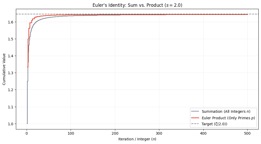
Euler found that this is equivalent to an infinite product that involves all the prime numbers.

オイラーは、この無限級数が、すべての素数を使った無限積と等価であることを発見しました。

$\displaystyle {\zeta(s) = \prod_{p \text{ prime}} \frac{1}{1 - p^{-s}} = \left(\frac{1}{1-2^{-s}}\right) \cdot \left(\frac{1}{1-3^{-s}}\right) \cdot \left(\frac{1}{1-5^{-s}}\right) \dots} \quad \text{for } s > 1$

The proof of this identity is fascinating. It essentially uses the Sieve of Eratosthenes—an ancient method for finding primes—translated into infinite algebra to sift out everything except the primes.

この恒等式の証明はとても面白くて、素数を見つける古典的な手法であるエラトステネスの篩を、無限の代数操作に置き換えて、素数以外をふるい落とすようなイメージです。

The proof of the Euler Product Formula

Below is a quick visualization of the two formulas over 500 iterations.

下は2つの式を500項まで繰り返して比較したものです。

Expanding to Complex Numbers

複素数への拡張

The fact that the summation and Euler’s product are equivalent suggests this function somehow “knows” the distribution of prime numbers. Riemann expanded this by using a complex number for $s$.

無限級数とオイラー積が等しいという事実は、この関数が素数の分布をどこかで知っているかのように見えます。リーマンはここから一歩進めて、$s$ を複素数として扱うように拡張しました。

When $Re(s) > 1$, the series converges and traces a clean spiral toward a specific point. When $Re(s) = 1$ or below, the standard summation diverges and shoots off the canvas. Click the graph on the left to choose a value of $s$ and see what happens.

$Re(s) > 1$（実部が1より大きい）では級数は収束し、ある点に向かってきれいなスパイラルを描きます。 $Re(s) = 1$ 以下では、通常の和は発散してしまい、図の外へ飛んでいきます。左側のグラフをクリックして $s$ の値を選び、動きを見てみましょう。

Riemann Hypothesis（リーマン予想）

Riemann’s claim is this:

リーマンの主張は次の通りです：

All non-trivial zeros of the Zeta function lie on a single vertical line where the real part is exactly 0.5.

ゼータ関数の「自明でない零点」はすべて、実部がちょうど 0.5 の一直線（垂直な直線）上に存在する。

It is known that the results converge to $0$ at $(-2, 0)$, $(-4, 0)$, $(-6, 0)$ and so on. These are called trivial zeros because it is fairly easy to prove that the function evaluates to zero at these points.

Non-trivial zeros are the other, harder-to-predict points where the function also vanishes. Riemann claims that all these points lie on a single line; this geometric symmetry would prove that prime numbers—though seemingly random—follow a strict, balanced distribution.

ゼータ関数は $(-2,0)$, $(-4,0)$, $(-6,0)$ …（負の偶数）で $0$ になることが知られており、これらは比較的簡単に示せるため「自明な零点」と呼ばれます。

自明でない零点は、他にも存在する（より予測しづらい）ゼロ点です。リーマンは、これらの点がすべて一本の直線上に美しく整列していると予想しました。この幾何学的な対称性は、一見ランダムに見える素数の並びが、実は厳密で均衡のとれた規則に従っていることを意味します。

To explore values where the real part lies between 0 and 1, mathematicians use a related alternating sum, the Eta function, which keeps the results finite.

実部が0-1の範囲を調べるために、数学者は関連する交代級数、エータ関数を使います。これは値を有限に保ってくれます。

This makes a stabilized version of the Zeta function that alternates signs to create a “zig-zag” convergence. This allows the series to match the Zeta function for $Re(s) > 1$ while remaining finite in the critical region below.

これは符号を交互に入れ替えることでジグザグに収束させ、ゼータ関数を安定化したものとして機能するイメージです。これを使うと、級数は $Re(s) > 1$ ではゼータ関数と一致しつつ、それ以下でも発散せず有限の値として扱えます。

$\displaystyle \eta(s) = \sum_{n=1}^{\infty} \frac{(-1)^{n-1}}{n^s} = 1 - \frac{1}{2^s} + \frac{1}{3^s} - \frac{1}{4^s} + \dots$

$\displaystyle \zeta(s) = \frac{1}{1 - 2^{1-s}} \eta(s)$

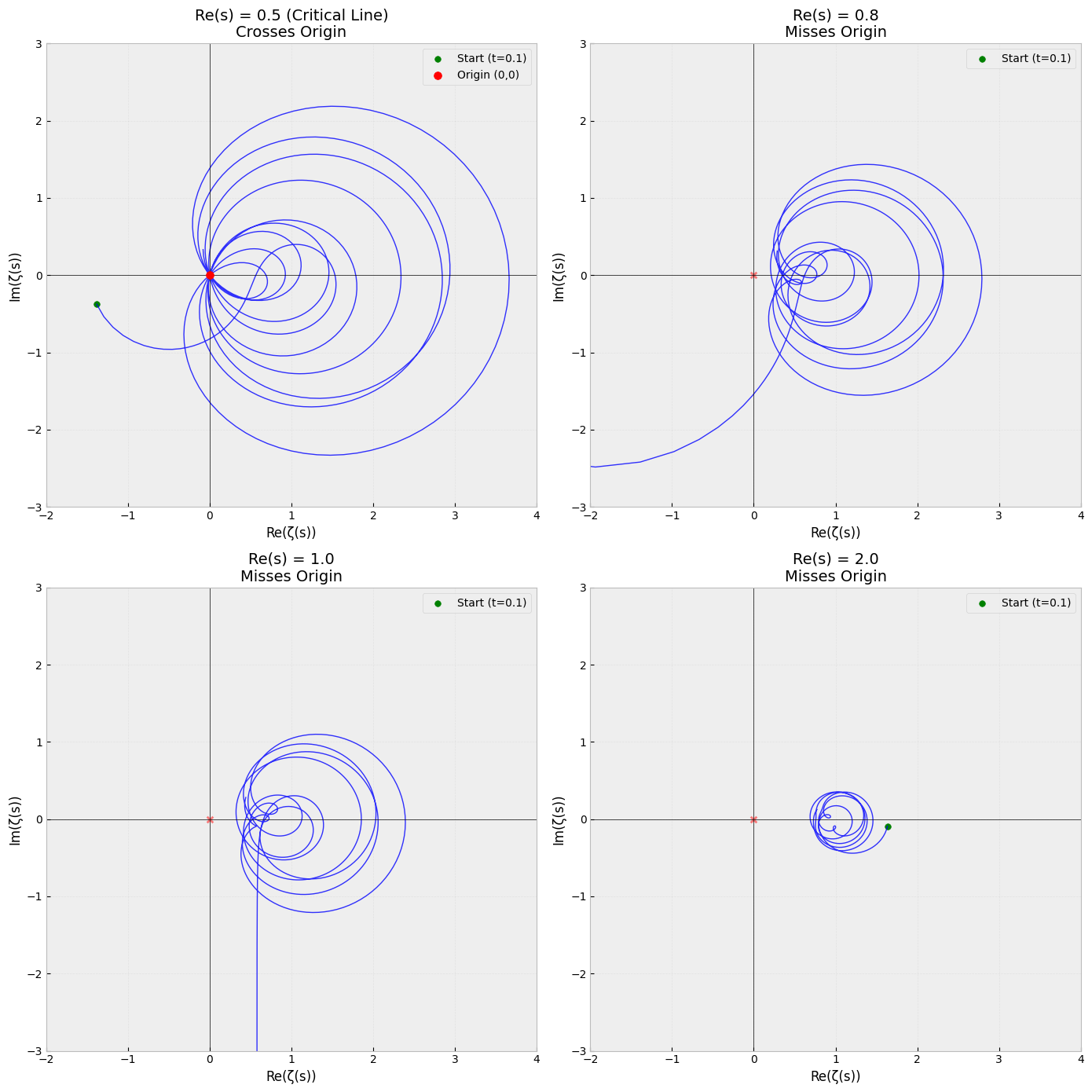
Using this, we can visualize Riemann hypothesis. The demo below shows how the output changes as we increase the imaginary part. On the left is the input ($s$), and on the right is the output. When the input lies on the line $Re(s) = 0.5$, the resulting spiral passes through the origin ($0,0$) multiple times.

これでリーマン予想を可視化できます。下のデモでは虚部を増やしたときに出力がどう変わるかを示しています。左が入力（$s$）、右が出力です。入力が $Re(s)=0.5$ の直線上にあると、出力のスパイラルは原点（$0,0$）を何度も通過します。

The result may look wiggly when $Re(s)$ is small. This is due to limited precision, since we need to stop the calculation at a certain point. For more accurate results, see the graphs below, drawn with Python.

$Re(s)$が小さいと結果の線がよれて見えますが、これは計算をある程度で打ち切っているので精度に問題があるからです。より正確な結果は、Pythonで描いた下のグラフを見てください。