Continuous Mapping 連続的な写像

Linear mapping

線形写像

The simplest example of continuous mapping is transforming one range of numbers into another while preserving proportional relationships. This is called linear mapping, and we use it all the time in programming.

連続的な写像の最も簡単な例は、ある数値の範囲を別の範囲へと、比例関係を維持したまま変換することです。プログラミングでは線形写像はそこらじゅうで使われています。

Conversion from Celsius to Fahrenheit is a good example of a linear mapping. You’d want to map 0°C to 32°F and 100°C to 212°F.

摂氏から華氏への変換は線形写像の良い例です。0°Cを32°Fに、 100°Cを212°Fに対応させます。

This can be written as:

これは下のように書けます。

$\begin{aligned} F = \frac{9}{5}C + 32 \end{aligned}$

$C$ is the temperature in Celsius
$F$ is the temperature in Fahrenheit
$C$ は摂氏の温度
$F$ は華氏の温度

This equation can be seen as a calculation for conversion, but it can also be viewed as a relationship that maps Celsius and Fahrenheit notations one-to-one. Since 100°C and 212°F indicate exactly the same thing, it makes sense to think of them as different names for the same thing rather than as a conversion.

この式は計算による変換として見ることもできますが、摂氏の表記と華氏の表記を1対1に対応させる関係を示したものとして見ることもできます。実際100°Cと212°Fは全く同じものを示しているので変換というよりは同じものの別の名前として考えてもしっくりきます。

Linear Mapping Formula

線形写像の公式

More generally, linear mapping can be written as below. Try if you can get the temperature conversion formula above by substituting with actual numbers.

より一般的に、線形写像は下のように表せます。実際の数値を代入して、上の温度を変換する式が得られるか試してみましょう。

$\begin{aligned} y &= \frac{(x - a)}{(b - a)} \times (d - c) + c \end{aligned}$

Where:

$x$ is the input value.
$a$ , $b$ are the min/max values of the input range.
$c$ , $d$ are the min/max values of the output range.
$y$ is the mapped value in the new range.

ここで

$x$ は入力の値。
$a$ , $b$ は入力範囲の最小 / 最大値。
$c$ , $d$ は出力範囲の最小 / 最大値。
$y$ は新しい範囲に写像された値。

です。

Value to position

値から位置へ

Linear mapping is everywhere. Let’s say you are trying to visualize the progress of a project as a position of a character. The progress is a value between 0 and 100, and your character should walk from the left side of the screen to the right side.

Try moving the slider in the demo below and see how the character (the circle!) moves accordingly. ThelinearMap()function implements the formula above. ThewithinBounds parameter determines whether to constrain the output value within the range of the min/max or stretch beyond.

線形写像はあらゆる場所で使われています。例えば、プロジェクトの進捗状況をキャラクターの位置として視覚化します。進捗は0から100の間の値で、キャラクターは画面の左端から右端まで歩くことになります。

下のデモでスライダーを動かすと、キャラクター（ただの円です）がそれに応じて動きます。linearMap()関数は上の公式の実装で、withinBoundsパラメータは、出力値を最小値 / 最大値の範囲内で制限するか、その範囲を超えて伸ばすかを決めます。

function linearMap(x, a, b, c, d, withinBounds = false) {
  let y = (x - a) * (d - c) / (b - a) + c;
  
  if (withinBounds) {
    return Math.min(Math.max(y, Math.min(c, d)), Math.max(c, d));
  }
  return y;
}

Again, this can be seen as a mere calculation, but it can also be seen as a mapping or representation. The value 0 stands for the left side, and 100 stands for the right side. Mapping helps you to grasp and handle the position more intuitively than by directly dealing with the coordinate.

これはただの計算としても、写像または数値による表現として見ることもできます。0は左端を、100は右端を表しています。写像を使うことで、座標を直接使うよりも直感的に位置を把握し扱うことができます。

Because this is such a common operation, p5.js has its own map() function. Try replacing the linearMap() with the map() and it still works exactly the same.

これはとても一般的な操作なので、p5.jsには独自のmap()関数が用意されています。linearMap()をmap()に置き換えて、全く同じように動くことを確かめましょう。

Non-Linear mapping

非線形写像

Of course, mapping can be non-linear, meaning the values don’t change proportionally. Instead the changes can follow a curved pattern, accelerating or decelerating.

もちろん、写像は非線形、つまり、値の比例による一定の変化ではなく、加速したり減速したりするような曲線的な変化である場合もあります。

Easing functions are good examples. Let’s update the map function. Try dragging the slider again and see how it feels different. The circle goes faster in the middle and slower around the edges.

イージング関数はその良い例です。写像関数を書き換えてみましょう。下のスライダーを操作すると、動きの感じ方が違うことが分かります。円は中央部分で速く、端に近づくにつれてゆっくりと動きます。

Affine transformation

アフィン変換

We have looked at examples of linear and non-linear mapping in one dimension. If you think of these as mappings between a 1D space to another 1D space, the natural next step is to expand to higher dimensions.

ここまでは1次元の線形写像と非線形写像の例を見てきました。これらを1次元空間から別の1次元空間への写像と考えれば、より高次元へと拡張するのが自然な次のステップでしょう。

Mapping a Point in 2D Space

2次元空間での点の写像

What if we mapped a point in a 2D space to another point in 2D space? One of the most common ways of doing this is called affine transformation, and it’s widely used for transforming shapes.

2次元空間上の点を別の2次元空間上の点に写像するとどうなるでしょう。最も一般的な方法の1つは、形の変換に広く使わるアフィン変換です。

Let’s look at the demo first to see what it does. Try moving your mouse to see the shape changes.

まずはデモを見て、動作を確認してみましょう。マウスを動かして形が変化する様子を見てください。

The Affine Transformation Formula

アフィン変換の式

The magic happens in the applyTransformation() function. It takes a matrix that defines the transformation and applies it to a point.

変換の魔法はapplyTransformation()関数の中で起こります。この関数は変換を定義する行列を受け取り、それを点に対して適用します。

The transformation can be written as:

この変換は下のように表せます。

$\begin{bmatrix} x' \\ y' \\ 1 \end{bmatrix} = \begin{bmatrix} a & b & e \\ c & d & f \\ 0 & 0 & 1 \end{bmatrix} \begin{bmatrix} x \\ y \\ 1 \end{bmatrix}$

Here, $x$ and $y$ are the original coordinates, $x′$ and $y′$ are the transformed coordinates. The 1s below the coordinates and the third row (0,0,1) under matrix may look arbitrary, but this is a trick that makes it possible to include translation as part of the transformation. This is called homogeneous coordinates.

ここで、 $x$ と $y$ は元の座標、 $x′$ と $y′$ は変換後の座標です。座標の下にある1と行列の3行目（0,0,1）は一見、恣意的に見えますが、これは平行移動を変換の一部として含めるための工夫です。これを同次座標と呼びます。

Homogeneous coordinates represent points in space using an extra dimension. In the affine transformation formula above, this extra dimension lets us add arbitrary values to x and y.

同次座標は空間内の点を表現するために1つ追加の次元を用います。上のアフィン変換式では、この追加の次元のおかげでxとyに任意の値を加えることができます。

In homogeneous coordinates, scaling all coordinates by the same nonzero factor results in the same spatial point. I.e., for any $k ≠ 0$ , $(x, y, w)$ and $(kx, ky, kw)$ represent the same point.

同次座標では、すべての座標をゼロ以外の同じ係数で拡大縮小しても空間上の同じ点を表します。つまり、任意の $k≠0$ に対して、 $(x, y, w)$ と $(kx, ky, kw)$ は同じ点を表します。

In affine transformations, w is typically fixed at 1, so this scaling property isn’t used. But having a variable w becomes very handy in more complex transformations, like 3D projection, where dividing by w introduces depth effects.

アフィン変換では、通常 $w$ は1に固定されるため、この拡大縮小の性質は使われません。ですが、可変の $w$ は3Dプロジェクションのようなより複雑な変換では、wで除算することで奥行き効果を生み出すのに非常に便利になります。

We can separate $x$ and $y$ if this is easier for you. As an exercise, try assigning random values to the matrix, and transforming multiple points with the same matrix manually. Doing this on paper will help build the intuition.

式を $x$ と $y$ に分けて書くと分かりやすいかもしれません。練習のため、行列にランダムな値を入れて、同じ行列で複数の点を手作業で変換してみましょう。紙の上で計算すると、より直感的に理解できます。

$x' = a x + b y + e$

$y' = c x + d y + f$

Types of 2D Affine Transformations

様々な2次元アフィン変換

You can create different kinds of transformations by changing the matrix values. You can even combine them by multiplying matrices together.

行列の値を変えることで、様々な種類の変換を作ることができます。さらに、行列を掛け合わせることで複数の変換を組み合わせることも可能です。

Scaling

拡大縮小

To scale a shape by $sx$ in the x-direction and $sy$ in the y-direction:

x方向に $sx$ 、y方向に $sy$ で形状を拡大縮小する。

$\begin{bmatrix} sx & 0 & 0 \\ 0 & sy & 0 \\ 0 & 0 & 1 \end{bmatrix}$

Rotation

回転

To rotate a shape by $\theta$ degrees:

図形を $\theta$ 度回転させる。

$\begin{bmatrix} \cos\theta & -\sin\theta & 0 \\ \sin\theta & \cos\theta & 0 \\ 0 & 0 & 1 \end{bmatrix}$

Translation

平行移動

To move (translate) a shape by $tx$ in x and $ty$ in y:

x方向に $tx$ 、y方向に $ty$ だけ形状を移動する。

$\begin{bmatrix} 1 & 0 & tx \\ 0 & 1 & ty \\ 0 & 0 & 1 \end{bmatrix}$

Shear

せん断

To shear the shape in the x or y direction:

x方向またはy方向に形状をせん断（斜めに傾けるように変形）する。

$\begin{bmatrix} 1 & sh_x & 0 \\ sh_y & 1 & 0 \\ 0 & 0 & 1 \end{bmatrix}$

Let’s look at another demo. This is almost identical to the demo above, but it translates and rotates the shape instead of skewing. Can you try editing the code to use other types of transformations?

別のデモを見てみましょう。これは上のデモとほぼ同じですが、歪曲ではなく、図形の平行移動と回転を行います。コードを編集して、他の種類の変換も試しましょう。

We have another example in GLSL below. Since GLSL supports matrices natively, it is easy to multiply them and apply multiple transforms. Play around with this code too.

下はGLSLを用いた例です。GLSLは行列を標準でサポートしているので、行列の掛け合わせて複数の変換を簡単に適用できます。このコードでも色々試してみましょう。

Radial Basis Function (RBF) Interpolation

放射基底関数（RBF）補間

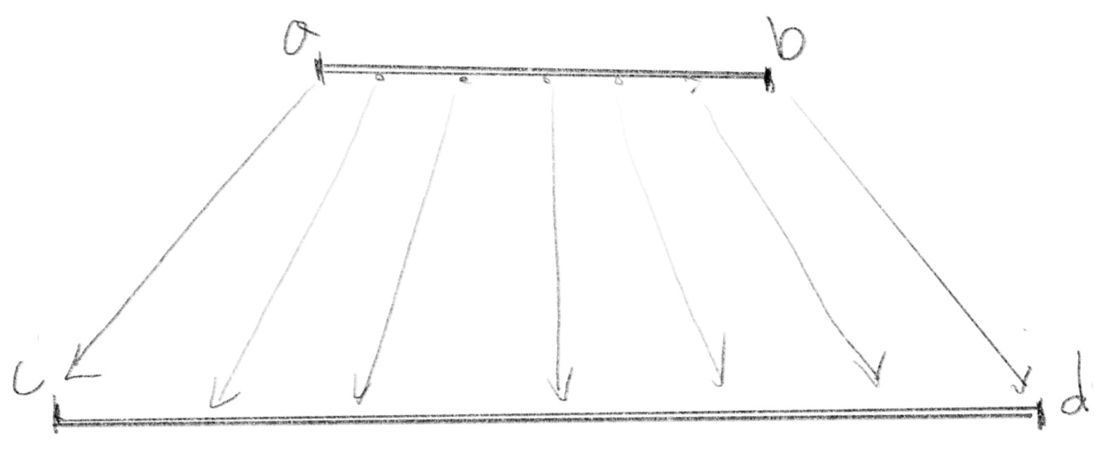
Affine transformation is a powerful tool for mapping between two spaces, but it is limited to linear transformations. What if you need a more arbitrary, nonlinear mapping? Radial Basis Function (RBF) Interpolation is one of the best solutions.

アフィン変換は2つの空間の間の写像を行う強力なツールですが、線形変換に限られています。より自由な非線形写像が必要な場合はどうすれば良いでしょう。放射基底関数（RBF）補間は最適な解決策の1つです。

RBF interpolation provides a way to smoothly estimate values across scattered data points. In other words, if you have multiple pairs of corresponding points, you can derive a mapping that accurately reflects those key points while smoothly interpolating the values in between.

RBF補間は、散在するデータ点全体の値を滑らかに推定できる手法です。複数の対応点のペアがあれば、このキーとなる点を正確に反映しながら、その間の値を滑らかに補間する写像を作り出すことができます。

If there are only two key pairs, this can be easily solved by a linear interpolation. But it gets tricky when there are a lot more key pairs. Instead of linear interpolation, RBF uses a weighted influence of known points to estimate unknown values.

キーとなる点のペアが2組だけの場合は、線形補間で簡単に解決できますが、ペアが多くなると複雑になります。線形補間の代わりに、RBFは既知の点がどれだけ結果に影響を及ぼすかを重み付けして未知の値を推定します。

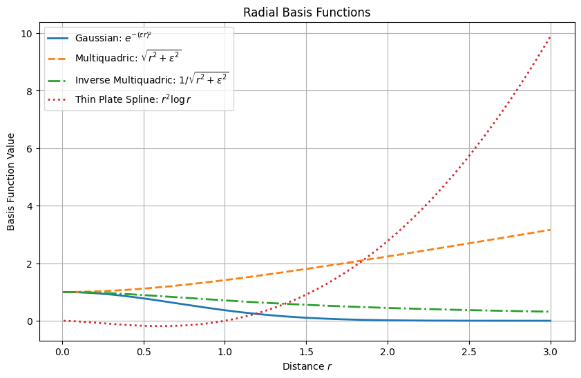
The function to calculate the influence of each point is called a radial basis function, and different functions can be used. A radial function is a function of the distance $r$ between a point and a key point, and returns the weight that represents the influence of the key point. Below are a few examples of common functions.

それぞれ点の影響を計算する関数は放射基底関数（RBF）と呼ばれ、様々な関数を使用することができます。放射基底関数は、ある点とキーとなる点の間の距離 $r$ の関数で、キーの影響を表す重みを返します。一般的な関数の例をいくつか以下に示します。

Google Colab

Let’s see RBF interpolation in action. Drag the white points in the demo below to deform the shape as you want.

実際のRBF補間の動作を見てみましょう。下のデモで白い点をドラッグして、好きなように変形させてください。

If you look at the code, you will notice that the RBFInterpolator precomputes the weights rather than directly taking the weighted average of the key points. This is for two purposes:

コードを見ると、RBFInterpolatorはキーポイントの重み付き平均を直接取るのではなく、重みを事前計算していることに気付くでしょう。これには2つの目的があります。

1. Performance: To make it more performant

2. Exact Mapping: Solving for weights ensures that the interpolation exactly matches the key points.

パフォーマンス: 処理を高速化
正確な写像: 補間の結果がキーとなる点と正確に一致するような重みの値を得る

computeWeights() is the function to precompute the weights. In this function:

computeWeights()が重みを事前に計算するための関数です。この関数は以下の計算を行います。

A is a matrix that stores the radial function values between all key points in the original space. i.e., If we call these points $o_0$ , $o_1$ , $o_2$ , …, then A[0][0] represents the radial function applied to the distance between $o_0$ and itself, A[0][1] is between $o_0$ and $o_1$ , and so on.
f is a matrix that stores the key points in the destination space, separated by dimension. i.e., If the original point $o_0$ maps to $d_0$ , f[0][0] is the x-coordinate of $d_0$ , and f[0][1] is the y-coordinate.
Then for each dimension, solveLinearSystem() solves a system of equations to find weights that ensure the interpolation exactly preserves all key points.
Aは元の空間における全てのキーの間のRBFの値を格納する行列です。つまり、これらの点を $o_0$ 、 $o_1$ 、 $o_2$ 、…と呼ぶと、A[0][0]は $o_0$ と自身との間の距離にRBFを適用した値、A[0][1]は $o_0$ と $o_1$ の間、というように表されます。
fは結果となる空間でのキーを次元ごとに分けて格納する行列です。つまり、元の点 $o_0$ が $d_0$ に写像される場合、f[0][0]は $d_0$ のx座標、f[0][1]はy座標となります。
solveLinearSystem()は連立方程式を解いて、補間の結果がそれぞれの次元について全てのキーを正確に再現するような重みを見つけます。

This means we are solving the following system of equations:

これは以下の連立方程式を解くことを意味します。

$A_{0,0} w_0 + A_{0,1} w_1 + A_{0,2} w_2 + \dots + A_{0,n} w_n = f_{0,d}$
$A_{1,0} w_0 + A_{1,1} w_1 + A_{1,2} w_2 + \dots + A_{1,n} w_n = f_{1,d}$
$\vdots$
$A_{m,0} w_0 + A_{m,1} w_1 + A_{m,2} w_2 + \dots + A_{m,n} w_n = f_{m,d}$

$w_j$ are the weights we are solving for.
$w_j$ は、求める重み。

Using the precomputed weights, interpolate() returns the interpolated value for a given input point. It applies the radial basis function to the distance between the input and each key point, multiplies the result by the corresponding weight to get its influence, and sums up all influences to produce the final result. If the input is one of the key points in the original space, these weights guarantee that the result is exactly the corresponding key point in the destination space.

事前計算された重みを使って、interpolate()は入力された点に対する補間の結果を返します。この関数は、入力とそれぞれのキー間の距離にRBFを適用し、対応する重みを掛けて影響の大きさを計算し、全ての影響を合わせて結果を求めます。入力が元の空間のキーと一致する場合、これらの重みによって、結果が結果となる空間の対応するキーと完全に一致することが保証されます。

The solveLinearSystem() function implements Gaussian elimination with partial pivoting to solve the system of linear equations.

solveLinearSystem()関数はピボット選択を用いたガウスの消去法によって連立一次方程式を解きます。

Gaussian Elimination ガウスの消去法

Note that even if all the key points are mapped to the same points (i.e., identity mapping at key points), the RBF interpolation can still deform the shape (or the space) other than these key points.

キーとなる点が全て同じ点に写像される場合（つまりキー点で恒等写像となる場合）でも、RBF補間はキー点以外の形状（または空間）を歪ませることがあるので注意してください。

RBF interpolation is a very powerful tool for making a mapping system that follows a given set of data points, especially when we are trying to predict something for which we don’t have clear logic or explanation, such as choices made by people or natural phenomena.

RBF補間は、データ内の点の集合に従って写像システムを構築できる強力なツールです。特に、人々の選択や自然現象など、明確な論理や説明が存在しない対象の予測に効果を発揮します。