Parametric Approaches パラメトリックアプローチ

While the cumulative approach is straightforward and versatile in theory, it is often not the best for many practical use cases where you want more precise control over the overall shape and details, such as in drawing or design tools.

積み重ねによるアプローチは理論上は素直で汎用的ですが、描画ツールやデザインツールなど、実際の利用シーンで、全体の形や細部をより正確に制御したい場面では必ずしも最適ではありません。

These tools usually adopt parametric approaches. In the parametric approach, a shape or curve is defined mathematically using one or more parameters. By varying these parameters, you can generate points that make up the shape. For example, if the parameter is called $t$, you can get all the points from beginning to end by moving $t$ within a certain range.

これらのツールは大抵、パラメトリックなアプローチが用いられます。パラメトリックアプローチでは、形や曲線は1つまたは複数のパラメータを使って数学的に定義され、これらのパラメータを変化させることで、形状を構成する点を生成します。例えばパラメータを $t$ とすると、この $t$ を $[0, 1]$といった一定の範囲内で変化させることで、始めから終わりまでのすべての点を取得することができます。

The most commonly used parametric curve that you probably know is the Bézier curve. But before jumping into it, let’s go through several examples to get used to the idea of the parametric approach.

ベジエ曲線は最も一般的に用いられるパラメトリックな曲線です。おそらくこれを読んでいる方もご存知でしょう。しかしベジェ曲線に踏み込む前に、いくつかの例を見てパラメトリックなアプローチに慣れていきましょう。

Line Segment

線分

Starting from the simplest example - a straight line segment (not a curve!) A straight line segment between two points $(x_1,y_1)$ and $(x_2, y_2)$ can be parameterized as follows:

（曲線ではありませんが）最も単純な例として線分から始めましょう。 2点 $(x_1,y_1)$ と $(x_2, y_2)$ の間を結ぶ線分はパラメータを用いて下のように表すことができます。

$x(t) = (1-t)x_1 + tx_2$
$y(t) = (1-t)y_1 + ty_2$

Take a look at the demo below.

デモを見てみましょう。

This is a linear interpolation between two-dimensional points.

これは2次元の点の間の線形補間です。

const t = (frameCount % cycle) / (cycle - 1);

This line causes the t to cycle from 0 to 1 over cycle frames. Meanwhile, the following lines move xt and yt from (x1, y1) to (x2, y2) as t progresses.

この行は、tが0から1にcycleフレームをかけて循環するようにします。そして次の行ではtが進むにつれてxtとytを(x1, y1)から(x2, y2)に移動させます。

const xt = x1 * (1 - t) + x2 * t;
const yt = y1 * (1 - t) + y2 * t;

Circle

円

A classic example of a parametric shape is a circle with radius $r$ centered at the origin:

原点を中心とする半径 $r$ の円は、パラメトリックな形状の古典的な例です。

$x(t) = r \cos(t)$
$y(t) = r \sin(t)$

Rotation and Trigonometry 回転と三角関数

Here, $t$ ranges from $0$ to $2 \pi$. As $t$ varies, the values of $x(t)$ and $y(t)$ trace out the points on the circle.

$t$ の範囲は $0$ から $2 \pi$ です。$t$ が変化するにつれて、$x(t)$ と $y(t)$ の値が円上の点を描き出します。

Lissajous Curve

リサージュ曲線

By modifying the formula for a circle a bit, you can create more complex and interesting shapes called Lissajous curves. You can think of a circle as a special case of a Lissajous curve, or a Lissajous curve as a circle-like shape with the horizontal and vertical movements out of sync. In general, it is described as combining two perpendicular simple harmonic motions (which are sine curves or the oscillation that a spring makes) in the x and y directions of different frequency.

円の公式を少し書き換えると、リサージュ曲線と呼ばれる、より複雑で面白い形を作ることができます。円をリサージュ曲線の特別なケースと考えることも、リサージュ曲線を水平と垂直の動きが同期していない円に似た形と考えることもできます。一般的に、リサージュ曲線は周波数が異なるx方向とy方向の2つの垂直な単振動（サインカーブ、またはバネが作る振動）の組みわせとして表されます。

$x(t) = A \sin(at + \delta)$
$y(t) = B \sin(bt)$

Here, $A$ and $B$ are the amplitudes, $a$ and $b$ are the frequencies, and $\delta$ is the phase difference. The parameter $t$ usually ranges over a few cycles, such as $[0, 2\pi]$ or $[0, 4\pi]$.

$A$ と $B$ は振幅、$a$ と $b$ は周波数、$\delta$ は位相の差です。通常、パラメータ $t$ は何周かにわたり、例えば $[0, 2\pi]$ や $[0, 4\pi]$ などの範囲で変化します。

Compare the demo below with the circle demo above. You can randomize the values of A, B, a, b, and delta by clicking on the canvas to draw different Lissajous curves.

下のデモを、上の円のデモと比べてみましょう。キャンバスをクリックすることで A、B、a、b、 delta の値をランダムに選び、異なるリサージュ曲線を描くことができます。

https://en.wikipedia.org/wiki/Lissajous_curve#/media/File:Lissajous_animation.gif CC BY-SA 3.0

Easing curves

イージングカーブ

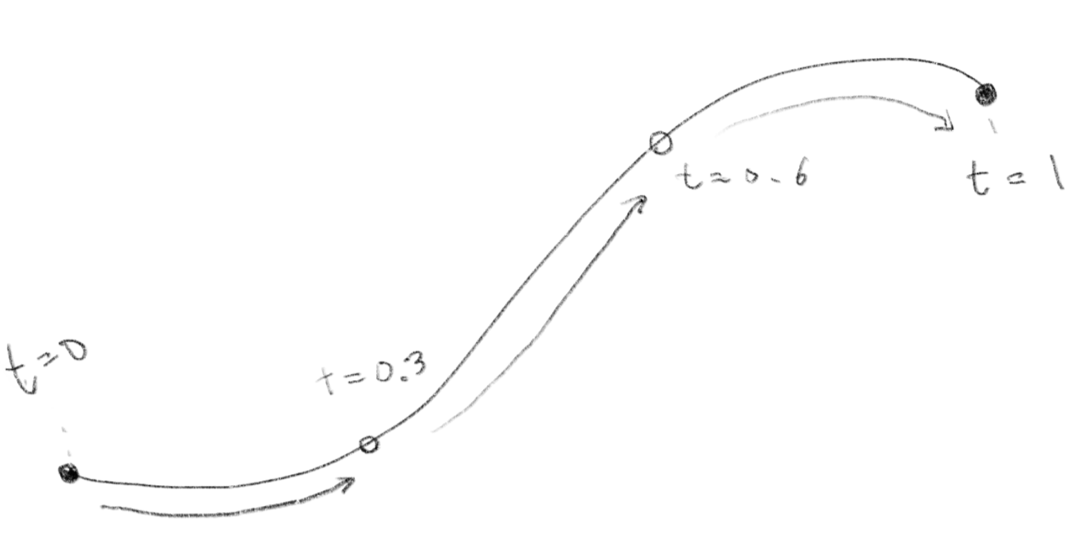
Easing curves that we often use in animations are also great examples of parametric curves. Although for animations the parameter $t$ is usually associated with time, not with a spatial coordinate, you can clearly see that these functions create different curves if we plot t and the returning values on a graph.

アニメーションでよく用いられるイージングカーブも、パラメトリックな曲線の良い例です。アニメーションの場合、パラメータ $t$ は通常、空間座標ではなく時間に割り当てられますが、グラフに $t$ と戻り値をプロットすると、これらの関数が異なる曲線を生み出すことがはっきりみて取れます。

If $f(t)$ is an easing function, strictly speaking, here the curve is defined as a combination of two functions.

$f(t)$がイージング関数とすると、厳密に言えば、ここでは曲線を2つの関数の組み合わせとして定義していることになります。

$x = t$

$y = f(t)$

On the next page, we’ll learn how to draw arbitrary shapes more freely.

次のページでは、より自由に任意の形状を描く方法を学びます。

Bézier and Spline ベジェとスプライン