Fourier Series フーリエ級数

Fourier transform

フーリエ変換

In Sine Waves and Additive Synthesis, we added up a series of sine waves to create waves with different shapes. For example, a square wave can be expressed as a combination of sine waves as shown below. This type of series is called Fourier series.

サイン波と加算合成のページではいくつものサイン波を足し合わせて様々な形の波を作りました。例えば矩形波は下のようなサイン波の組み合わせとして表すことができます。このような級数はフーリエ級数と呼ばれています。

${\displaystyle {\begin{aligned}x_{\text{square}}(t)&={\frac {4}{\pi }}\sum _{k=1}^{\infty }{\frac {\sin \left(2\pi (2k-1)ft\right)}{2k-1}}\&={\frac {4}{\pi }}\left(\sin(2\pi ft)+{\frac {1}{3}}\sin(6\pi ft)+{\frac {1}{5}}\sin(10\pi ft)+\dots \right)\end{aligned}}}$

On this page, we convert an arbitrary function into a Fourier series. That is, given a function that represents a change in a certain quantity, such as the rectangular wave above, we decompose it into a series of sine waves.

このページでは任意の関数をフーリエ級数に変換します。つまりある数値の変化、例えば上の矩形波のようなものが関数として与えられた時に、それをサイン波の組み合わせに分解します。

Instead of delving too deeply into math, we will aim to create a drawing machine like the one below and gain some rough insights into how it works. A great thing about sketching with code is that you don’t need to fully understand a concept to start. Instead, you can start by tinkering with working examples and learn from the experience (And I’m learning a lot through writing this).

ここでは数学に深く踏み込む代わりに、下のようなドローイングマシンを作ることで、その仕組みについて大まかな洞察を得ることを目指します。素晴らしいことに、コードでスケッチを始めるのに概念を完全に理解する必要はありません。代わりに動作する例をいじり、その経験から学ぶことができます（そして、自分自身このページを書くことで学んでいます）。

We will only consider functions that can be expressed as a repetition of a constant period, such as square waves or the sketch below.

ここでは矩形波や下のスケッチのように元になる関数がある一定期間の繰り返しとして表せるもののみを考えます。

Fourier series is a basis for a little more complex concept called Fourier transformation. This extends the idea to non-periodic functions with an infinite range. Fourier transform is widely used in various fields such as sound processing, signal processing, and image compression. By applying Fourier transform to sound data, we can determine the amount of different frequencies contained within it. This lets us manipulate the data by reducing or increasing a certain range of frequencies.

フーリエ級数は、フーリエ変換と呼ばれるより複雑な概念の基礎になります。フーリエ変換は、無限の範囲を持つ周期的でない関数にまで同じ考え方を拡張するもので、音声処理、信号処理、画像圧縮など、さまざまな分野で広く使用されています。音のデータにフーリエ変換を適用すると、そこに含まれる異なる周波数の量が求められ、例えばある周波数範囲を減少させたり、増加させたりすることによって、データを操作することができます。

Adding up sine waves

サイン波を重ねる

Let’s take a moment to think about what it means to add up sine waves. The formula for the Fourier series looks like this (There are multiple ways to write essentially the same thing. You may see different versions in other materials.)

まずは、サイン波を加算するということが何を意味するのか考えてみましょう。フーリエ級数の式は次のようになります（他の資料では違うバージョンを見かけるかもしれません。本質的に同じことを書くための複数の方法があります）。

${\begin{aligned}FS(t)&=\sum _{k=0}^\infty a_k\cos (2\pi kt) + b_k\sin (2\pi kt)\end{aligned}}$

It may seem complicated, but this equation can be read as adding sine waves with different amplitudes ($a_k$, $b_k$) and different periods ($2\pi kt$ indicates that it revolves $k$ times while it goes from 0 to 1) from $k=0$ to $k=\infty$. Since the only difference between the sine and cosine waves is the starting point, we call them both sine waves. $\sum$ is the symbol for summation, and $\sum _{k=0}^\infty$ means to increment k from 0, 1, 2, 3, and so on, to infinity. and keep adding up the terms to the right. Note that $a_k$, $b_k$ can be zero, so it does not necessarily mean adding an infinite number of sine waves. Especially on computers, it always have to end somewhere since they can’t perform an infinite number of additions.

複雑に見えるかもしれませんが、この式は異なる振幅（$a_k$, $b_k$）と異なる周期（$2\pi kt$はtが0から1に進む間に$k$回転することを示しています）を$k=0$から$k=\infty$まで足し合わせると読むことができます。サインとコサインはスタート地点が異なるだけなので両方ともサイン波と呼びます。$\sum$は総和を表す記号で、$\sum _{k=0}^\infty$は、kを0から1、2、3、と無限大まで増やしながら右側の項を足し続けることを意味します。$a_k$, $b_k$はゼロでも良いので実際に無限個のサイン波を足すとは限りません。コンピュータでは無限回の足し算はできないので必ずどこかで打ち切りになります。

The demo below is an example of adding three different sine waves. It shows that complex waveforms can be created by combining simple waves.

下のデモは3つの異なるサイン波を足し合わせた例です。単純な波の組み合わせからより複雑な形の波が作れることがわかります。

If you’re wondering why we need both sine and cosine, take a look at the demo below. Adding a sine wave and a cosine wave with the same frequency but different amplitudes results in a sine wave with a different starting point (phase). Therefore, a pair of sine and cosine waves with the same frequency can be thought of as a way to express a single sine wave. In fact, you can write a pair in a single term using a complex number, but we won’t touch upon that now.

なぜサインとコサインの両方が必要なのでしょう。下のデモを見てください。周波数が同じで振幅が異なるサイン波とコサイン波を足すと、異なる開始点（位相）を持つサイン波が得られます。したがって、同じ周波数を持つ正弦波と余弦波のペアは、単一の正弦波を表す方法と考えることができます。実際、複素数を使うとこのペアを単一の項として書くことができるのですが、今は触れないでおきます。

Find the Fourier coefficients

フーリエ係数を見つける

Going back to the formula, $t$ is the argument of the function which is the horizontal axis in the demo above, and $k$ just increments from 0, so the only unknowns are the coefficients $a_k$ and $b_k$. What we need to do is to find the two arrays of numbers $a = [a_0, a_1, a_2, a_3…]$ and $b = [b_0, b_1, b_2, b_3…]$ that makes a function we want to recreate.

下の式に戻ると、$t$は関数の引数で上記のデモの横軸に相当し、$k$は単に0から増えていくだけなので、未知数は係数 $a_k$ と $b_k$ だけです。必要なのは、再現したい関数を作るための2つの数値配列 $a = [a_0、a_1、a_2、a_3…]$ と $b = [b_0、b_1、b_2、b_3…]$ を見つけることです。

${\begin{aligned}FS(t)&=\sum _{k=0}^\infty a_k\cos (2\pi kt) + b_k\sin (2\pi kt)\end{aligned}}$

Using code might be easier to understand. Fourier series can be written as follows, and the task is to find arrays a and b to pass to this function. Here, a and b are arrays of a finite number of numbers.

コードの方が分かりやすいかもしれません。フーリエ級数は下のように書くことができ、課題はこの関数に渡すaとbの配列を見つけることです。ここではaとbは有限個の数の配列です。

function fourierSeries(a, b) {
  return function result(t) {
    const cosTerms = a.map((an, n) => an * Math.cos(2 * Math.PI * n * t));
    const sinTerms = b.map((bn, n) => bn * Math.sin(2 * Math.PI * n * t));
    return cosTerms.reduce((sum, term) => sum + term, 0) + sinTerms.reduce((sum, term) => sum + term, 0);
  };
}

$a_k$ and $b_k$ can be obtained by calculating the definite integral of the corresponding $sin (2\pi kt)$ or $cos (2\pi kt)$ multiplied with the function $f(t)$ that we want to decompose. The range of t is from 0 to 1. We will discuss later why we are multiplying them by 2 or not based on whether k is 0..

$a_k$、$b_k$ は、分解したい元の関数 $f(t)$と対応する $sin (2\pi kt)$ または $cos (2\pi kt)$ を掛けて、定積分を計算すると求めることができます。tの範囲は0から1までとします。k が0かによって2を掛けたり掛けなかったりする理由には後で触れます。

${\begin{aligned} a_k =\int_{0}^{1} f(t) cos(2 \pi kt) dt = \int_{0}^{1} f(t) cos(0) dt\end{aligned}} \qquad if: k = 0$${\begin{aligned} a_k =2\int_{0}^{1} f(t) cos(2 \pi kt) dt \end{aligned}} \qquad if: k > 0$

${\begin{aligned} b_k =2\int_{0}^{1} f(t) sin(2 \pi kt) dt \end{aligned}}$

Definite integral and its approximation

定積分とその近似

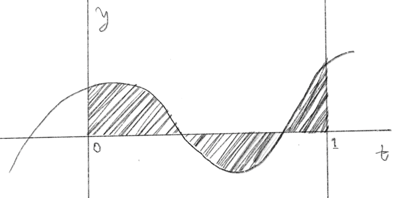
Explaining integrals would take up many pages, but here, let’s think of a definite integral as the area formed by the graph of a certain function. However, note that integrals can also take negative values. In the example below, the definite integral from $t = 0$ to $t = 1$ is obtained by subtracting the shaded area below the horizontal axis from the shaded area above the horizontal axis.

積分について説明するとそれだけで何ページにもなってしまいますが、ここでは非常に大雑把に定積分とはある関数のグラフが作る形の面積だと考えてください。ただし積分はマイナスの値もとります。下の例では $t = 0$ から $t=1$ までの定積分は横軸の上の斜線部分から下の斜線部分の面積を引いたものになります。

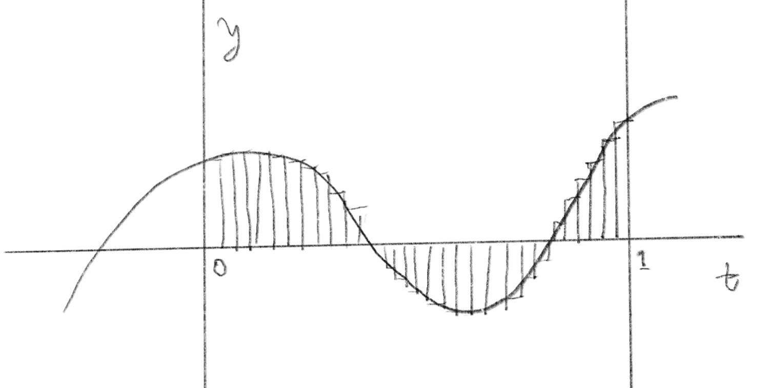
It is difficult to find the integrals of arbitrary functions in general, but it is easy to approximate them using code. You can simply divide the graph above into many small rectangles as shown in the drawing below. The more divisions you make, the more accurate the result will be. This is called a Riemann sum (you don’t have to remember it though).

一般に任意の関数の積分を求めるのは難しいのですが、コードを使うと簡単に近似することができます。上のグラフを下の図のように沢山の細かい長方形に分けてしまえば良いのです。分割の数を増やすほど、結果は正確になります。これはリーマン和と呼ばれています（覚えなくて大丈夫です）。

This is what it looks like when written in code. f is the function to be integrated, and N is the number of divisions.

コードで書くとこうなります。fは積分を取る対象の関数、Nは分割の数です。

function integral(f, N = 1000) {
  const dt = 1 / N;
  let sum = 0;
  for (let t = 0; t < 1; t += dt) {
    sum += f(t) * dt;
  }
  return sum;
}

Calculate the Fourier coefficients

フーリエ係数を計算する

We can implement the above formulas using this definite integral function. Pass the function to be decomposed into f, and specify how many a and b calculate with N.

この定積分関数を使って上の式を実装します。fには分解の対象になる関数を渡し、N で a と b を何個まで計算するか指定します。

function s(n) {
    return (t)=> Math.sin(2*Math.PI*n*t);
}

function c(n) {
    return (t) => Math.cos(2*Math.PI*n*t)
}

function fourierCoefficients(f,N) {
  const a = [];
  const b = [];

  for (let n = 0; n <= N; n++) {
    a.push(2 * integral(t=>f(t)*c(n)(t)));
    b.push(2 * integral(t=>f(t)*s(n)(t)));
  }
  a[0] /= 2
  return { a, b };
}

Demos!

デモ

We’re ready to go. First, let’s break down a square wave. The square wave can be written as this function.

これで準備ができました。まずは矩形波を分解してみましょう。矩形波はこんな関数で定義できます。

function square(t) {　return (t % 1) < 0.5 ? 1 : -1;　}

You can see that as N increases, it becomes closer to the square wave we are targeting.

Nを増やしていくと少しずつ目標とする矩形波に近づいていくのが分かります。

Let’s try with other functions. This is a sawtooth wave.

他の関数でも試してみましょう。これはノコギリ波です。

function sawtooth(t) { return (t % 1 - 0.5) * 2.0; }

How does this work?

なぜこれで上手くいくのか

Now that we have all the tools we need for sketching, you may be wondering why taking integrals can help us find coefficients. In this section, I will try to explain the background briefly. Feel free to skip if you are not interested, or if this rough explanation is not satisfactory, please refer to the materials at the end of the page.

これでスケッチのためのツールは出揃いましたが、なぜ積分を取ると係数が求められるのか不思議に思っているかもしれません。このパートではもう少しだけ背景を説明してみます。興味がなければスキップしても大丈夫ですし、この雑な説明では満足できない方はページの最後にある資料を参照してください。

Multiplying of sine waves

サイン波の掛け算

Let’s consider the product of two sine waves. Take a look the demo below. The result of multiplying two sine waves (A*B) is always greater than zero only when the phases are aligned, otherwise the areas above and below zero cancel each other out. As a result, if the phases are not aligned, the result of integration will be zero.

三角関数の積について考えてみましょう。下のデモを見てください。2つのサイン波を掛けた結果（A * B) は位相が揃っている時だけ全ての値が0より大きくなり、そうでない場合は0から上と下の面積が等しくなります。この結果、位相が揃っていない場合は積分した結果が0になります。

Finding the definite integral

定積分を求める

Let’s say there is a function f(t) that can be expressed as a Fourier series.

ある関数f(t)があって、この関数がフーリエ級数で表せるとします。

${\begin{aligned}f(t)&=\sum _{k=0}^\infty a_k\cos (2\pi kt) + b_k\sin (2\pi kt)\end{aligned}}$

$= a_0 cos(2 \pi 0t) + b_0 sin(2 \pi 0t) + a_1 cos(2 \pi 1t) + b_1 sin(2 \pi 1t) + a_2 cos(2 \pi 2t) + b_2 sin(2 \pi 2t) + …$

Due to what we saw above, if we multiply this function by, for example, $cos(2 \pi 2t)$, and integrate it, all terms except for $a_2 cos(2 \pi 2t)$ will disappear and become 0. The result will look as follows.. If you repeat this for both cos and sin, for all values of $k$, you will find $a_k$ and $b_k$.

上で見た理由によって、この関数に例えば$cos(2 \pi 2t)$を掛けて積分を取ると、なんと同じ形をしている$a_2 cos(2 \pi 2t)$ 以外の項が全て0になって消え得てしまい、結果は下記のようになります。これをcosとsinの両方、全ての$k$について繰り返すと$a_k$、$b_k$が得られることになります。

${\begin{aligned} \int_{0}^{1} f(t) cos(2 \pi 2t) dt = \int_{0}^{1} a_2\cos(2 \pi 2t)cos(2 \pi 2t) dt = \frac{a_2} {2} \end{aligned}}$

The integral $\int_{0}^{1} cos(2 \pi kt)cos(2 \pi kt) dt$ equals 1 when k is 0, and 1/2 for all other values of k. Similarly, $\int_{0}^{1} sin(2 \pi kt)sin(2 \pi kt) dt$ equals 0 when k is 0, and 1/2 for all other values of k. This is the reason why we need to change the formula based on whether k is 0 or not. Try drawing graphs to see why.

$\int_{0}^{1} cos(2 \pi kt)cos(2 \pi kt) dt$ はkが0の時だけ1、それ以外は1/2になります。同様に$\int_{0}^{1} sin(2 \pi kt)sin(2 \pi kt) dt$ はkが0の時に0、それ以外は1/2になります。これが理由でkが0かによって計算を変える必要があるのです。グラフを書きながら考えてみましょう。

As a vector space

ベクトル空間として考える

The other fascinating way to see this is to think about a Fourier series as a vector, and the integral of the multiplication of two sine waves as the inner product.

もう1つの非常に面白い見方は、フーリエ級数をベクトルとして考え、2つのサイン波の積の積分を内積として考えることです。

In a familiar vector space, such as a three-dimensional space, a vector can be decomposed into the magnitudes with respect to the directions of each basis, which defines the space, by taking the inner product (dot product) with the basis vectors, for example, (1, 0, 0), (0, 1, 0), and (0, 0, 1).

馴染みの深いベクトル空間、例えば三次元空間では、あるベクトルを、その空間を定める基底ベクトル、例えば（1, 0, 0), (0, 1, 0), (0, 0, 1) との内積（ドット積）を求めることで、それぞれの基底ベクトルの向きに対する大きさに分解することができます。

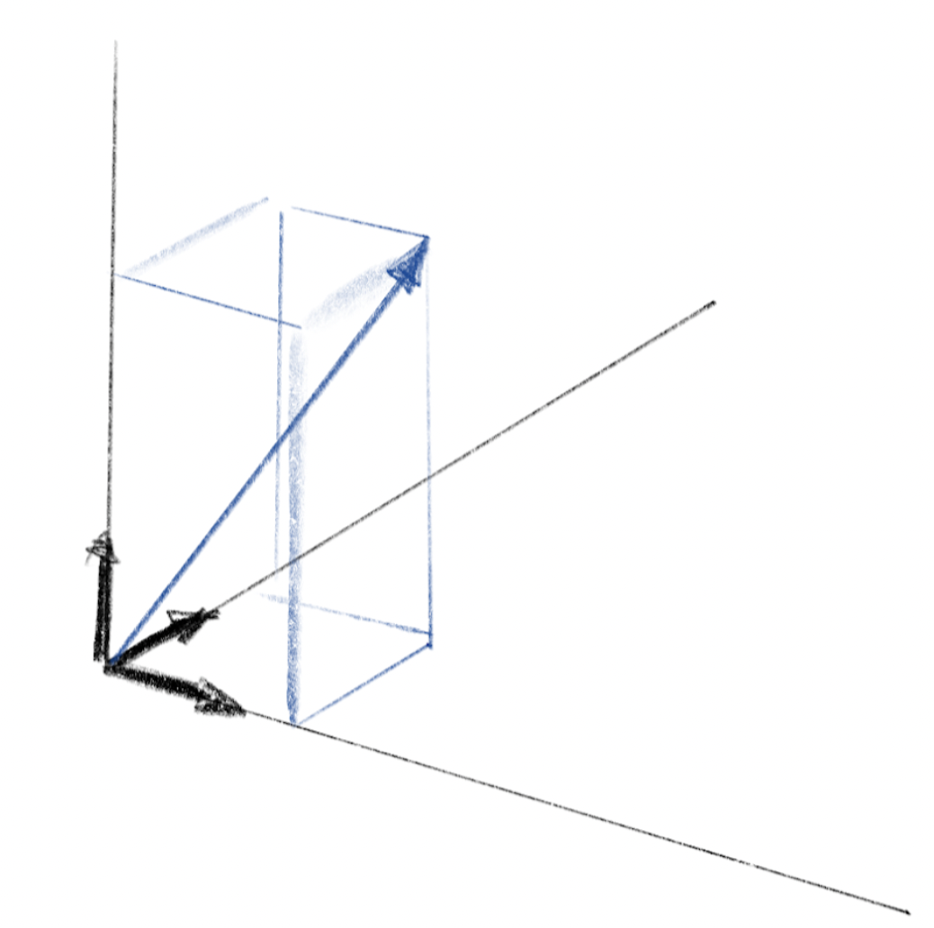
In mathematics, the concept of vector spaces can be expanded to sets of functions. In this case, a Fourier series given by $a_k cos(2πkt)$ and $b_k sin(2πkt)$ can be considered as a sum of basis vectors $cos(2πkt)$ and $sin(2πkt)$ multiplied by their respective magnitudes along each axis. As $k$ goes to infinity, this space has an infinite number of bases.

数学ではベクトル空間を関数の集合に拡張することができ、この場合$a_k cos(2 \pi k t)$、$b_k sin(2 \pi k t)$ で表されるフーリエ級数を、基底ベクトル $cos(2 \pi k t)$、$sin(2 \pi k t)$ にそれぞれの軸にそった大きさを掛けて足し合わせたものと考えることができます。$k$は無限大まで行くので、この空間には無限個の基底があることになります。

To calculate the inner product of vectors $a$ and $b$ in a multi-dimensional space, we multiply all the corresponding components and add them together (e.g. for 3 dimensions: $a_x b_x + a_y b_y + a_z b_z$). For functions, we can think of the integral, which sums up the return values for all inputs as the inner product.

多次元空間のベクトル$a$と$b$の内積を計算するには対応する成分を全て掛け合わせて足し合わせますが（例: 3次元の場合 $a_x b_x + a_y b_y + a_z b_z$）、関数の場合、全ての入力に対する戻り値を掛けて足し合わせたもの、つまり積分を内積とみなします。

The fact that the integral of the out-of-phase sine waves is zero corresponds to the dot product of different basis vectors being zero, which means they are orthogonal.

位相が揃ってないサイン波を掛けて積分すると0になるのは、異なる基底ベクトル同士のドット積を取ると0になり、これを直行と考えることに相当します。

To summarize, in the space of functions that can be represented by a Fourier series, the sine and cosine functions of different frequencies serve as the basis, and each function corresponds to a unique ‘point’ or ‘vector’ within this space. Converting a function into a Fourier series is to find the coordinates of that function in this space.

つまりフーリエ級数で表現できる関数の空間では、異なる周波数のサイン関数とコサイン関数が基底として機能し、各関数はこの空間内の一意な点またはベクトルに対応します。関数をフーリエ級数に変換することは、この空間で関数の座標を見つけることなのです。

Making a Drawing Machine

ドローイングマシーンを作る

We have gone quite abstract. Let’s back up and complete the drawing machine we saw at the beginning. We already have all the necessary tools. What’s left is to define the shape we want to draw as a function using Fourier series. Here, I defined the outline of the letter F as a function by converting SVG to an array.

だいぶ抽象的な話になりましたが、気を取り直して冒頭に見たドローイングマシーンを完成させましょう。必要な道具は全て揃っています。あと必要なのはフーリエ級数を使って描きたい形を関数として定義することです。ここではSVGを読み取って配列に変換することでFの文字のアウトラインを関数として定義しました。

To draw a 2D image, we will convert the x-axis and y-axis into Fourier series separately.

2Dの画像を描くので、x軸とy軸を分けてフーリエ級数に変換します。

xCoefs = fourierCoefficients((t) => shape(t).x, N);
fx = fourierSeries(xCoefs.a, xCoefs.b);
yCoefs = fourierCoefficients((t) => shape(t).y, N);
fy = fourierSeries(yCoefs.a, yCoefs.b);

To make what is happening clearly visible, plotFourierSeries is defined to draw circular motion on the canvas. This function will create a figure while performing the same calculation as the function that fourierSeries returns.

何が起きているのか目で見て分かるようにしたいので、plotFourierSeriese を定義して円運動をキャンバスに描くようにします。この関数はfourierSeries が戻す関数と同じ計算をしながら同時に図を作成してくれます。

Let’s take a look at the finished demo again. Try different shapes by rewriting the shape function.

もう一度完成したデモを見てみましょう。shape関数を書き換えて様々な形を試してみてください。

References

参考資料

Fourier series and Fourier transforms are one of the most important topics in the fields of mathematics and engineering, and studying them can go very deep. For those who want to learn more here is a list of resources that I looked at to write this page.

フーリエ級数とフーリエ変換は非常に奥深い、数学や工学の分野で最も重要なトピックの1つです。より深く知りたい方のためにこのページを書く参考にした資料を挙げておきます。

To move forward, it is useful to learn the representation of Fourier series using complex numbers. The first video provides a good visual introduction.

先に進みたい方は複素数を用いたフーリエ級数の表現について学ぶと良いでしょう。最初のビデオは良い導入になると思います。

Math for Programmers: 3D graphics, machine learning, and simulations with Python

Buy Math for Programmers: 3D graphics, machine learning, and simulations with Python on Amazon.com FREE SHIPPING on qualified orders

https://www.amazon.com/Math-Programmers-graphics-learning-simulations/dp/1617295353

数学ガールの物理ノート／波の重ね合わせ

Amazon.co.jp: 数学ガールの物理ノート／波の重ね合わせ eBook : 結城 浩: Kindle Store

https://www.amazon.co.jp/結城-浩-ebook/dp/B0B81QVC7Y/