Vibration and Propagation 振動と伝搬

In many cases, waves are caused by physical vibrations. With string instruments and percussions, you can actually see the parts of instruments such as wires, skins, wood, or metal trembling. When the vibration traverses through the air, it becomes a sound wave.

多くの波は物理的な振動によって起こります。弦楽器や打楽器では実際にワイヤーや皮、木や金属などのパーツが震えているのを見ることができます。この振動が空気に伝わることで音波になります。

Spring equation

バネ方程式

Let’s take a look at a spring as a simple model of vibration. The equation of a spring (Hooke’s law) is $F=-kx$, which means that when it’s extended or compressed, a force of the object to return to its original shape is proportional to the amount of deformation. If we ignore other factors, stretching and releasing a spring will create a perpetual oscillation. And if we plot this against time, we get a sine curve. This is called simple harmonic motion.

振動の簡単なモデルとしてバネをみてみましょう。バネの方程式（フックの法則）$F=-kx$ は、バネを伸ばしたり縮めたりしたときに物体が元の形に戻ろうとする力が変形された距離に比例していること示します。他の要因を無視すると、バネを伸ばして手を離せば永遠に続く振動が生まれることになります。この振動を時間軸にプロットするとサインカーブになります。これは単振動と呼ばれています。

Although the actual musical instruments are not as simple as this, spring is a good entry point for understanding the physics behind vibrations, such as the force of a string being pulled and returning with tension.

実際の楽器はここまで単純ではないのですが、弦が引っ張られて張力で戻る様子など振動の元になる物理を理解するのにバネは入り口になります。

Wave equation

波動方程式

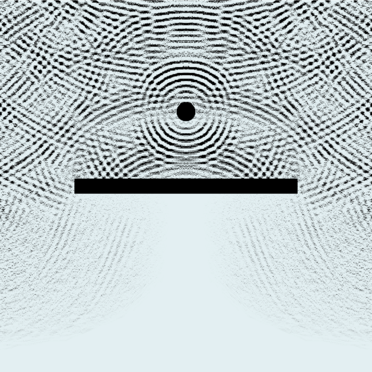
Next, let’s simulate the propagation of the vibration using the wave equation. We could use harmonic motion, but let’s use a noise function to make it slightly

次に振動が伝わる様子を波動方程式を使ってシミュレーションしてみます。単振動でも良いのですがノイズ関数を使ってもう少し面白くしてみます。

The one-dimensional equation of wave looks like this, with u representing the displacement of the wave. The left side is the second-order derivative with respect to time t, or how the rate of change is changing (in this case acceleration), and the right side is the second-order derivative with respect to position x.

1次元の波の方程式はこんな形で、uが波の変位を表します。左辺が時間tに関する2階微分、つまり変化量の変化量（この場合は加速度）、右辺が位置xに関する2階微分になっています。

${\displaystyle {\partial ^{2}u \over \partial t^{2}}=c^{2}{\partial ^{2}u \over \partial x^{2}}}$

We actually don’t need precise derivatives for the simulation on this page. The figure below shows how the demo is implemented. Please compare this diagram carefully with the explanation beneath. You can learn more about numerical approximation of derivatives on the Differentiation page.

実はこのページのシミュレーションでは厳密な微分は必要ありません。下の図がデモで使った実装方法です。この図とその下の説明をよく見比べてみてください。微分のページでは微分の数値的な近似についてもっと詳しく説明しています。

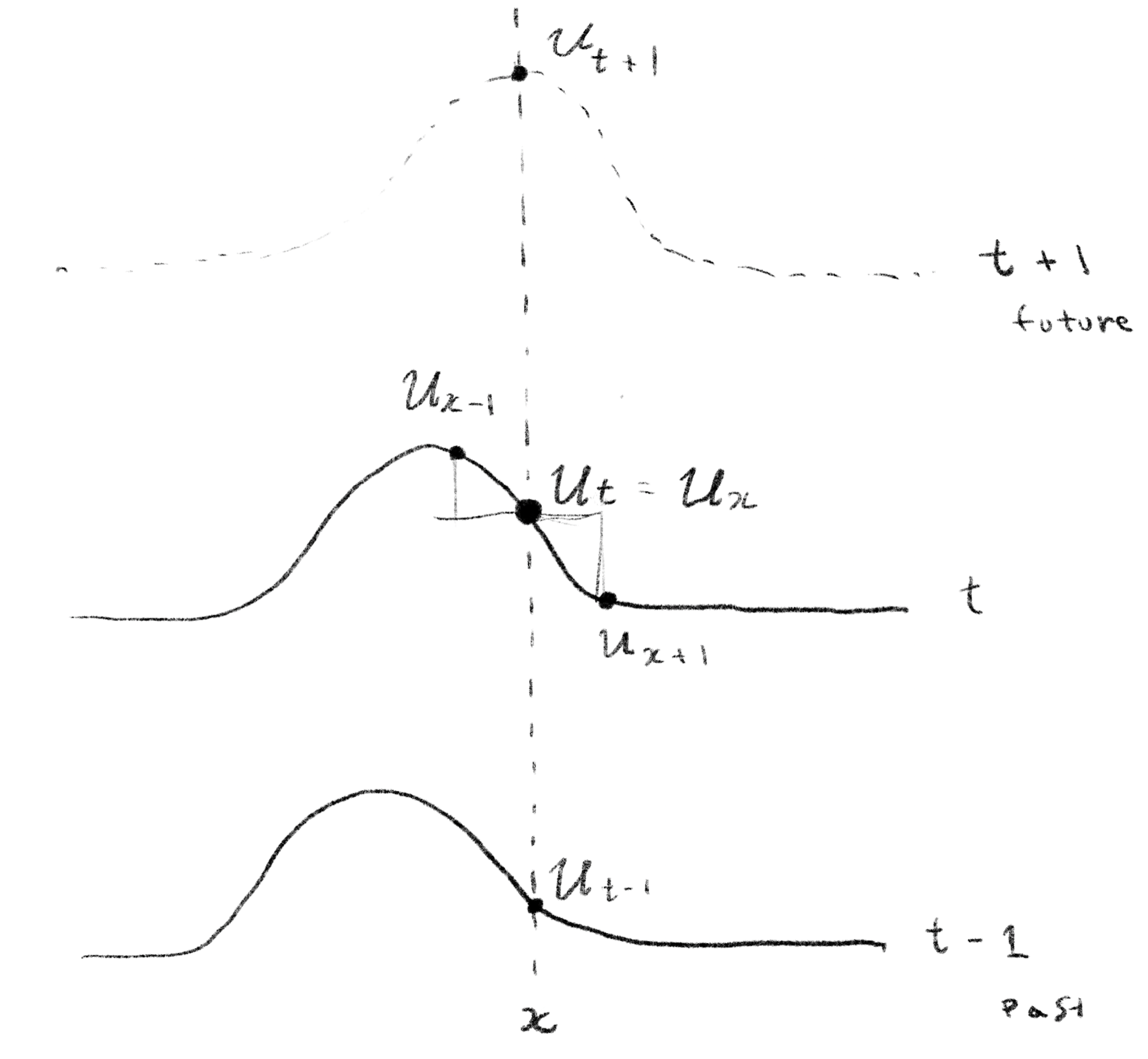
Since this does not have to be exact, we will approximate the derivative by sampling a suitably close times and locations and calculating the differences. For the left side, we can approximate the second-order derivative by subtracting the change from the value one frame back in the past to the current value$(u_t - u_{t-1})$, from the change from the current value to the value one frame ahead in the future$(u_{t+1} - u_t)$.

このシミュレーションは厳密でなくて良いので適当に近い時間や場所をサンプルして差を求めることで微分を近似することにします。すると左辺は1フレーム未来の値から現在の値を引いた変化量$(u_{t+1}-u_t)$から、現在の値から1フレーム前の値を引いた変化量$(u_t - u_{t-1})$を引くことで、2階微分を近似することができます。

$\dfrac{\partial^2u}{\partial t^2}\Rightarrow\;(u_{t+1}-u_t)\;-\;(u_t - u_{t-1})\;=\;u_{t+1}\;+\:u_{t-1\;}-\;2u_t$

Similarly, the right-hand side can approximate the second-order derivative by finding the differences between the current point($u_{x}$) and the next point to the left($u_{x-1}$), and the point to the right($u_{x+1}$) and the current point($u_{x}$), then calculating the difference between these differences.

同様に、右辺は現在の点($u_{x}$)と左隣の点($u_{x-1}$)、右隣の点($u_{x+1}$)と現在の点($u_x$)の差を求め、さらにそれらの差を計算することで2階微分を近似することができます。

$c^2\dfrac{\partial^2u}{\partial x^2}\Rightarrow\;c^2\left[(u_{x-1}-u_x)\;-\;(u_x - u_{x+1})\right]\;=\;c^2(u_{x-1}\;+u_{x+1\;}-\;2u_x)$

The equation can be transformed to find the value of $u$ one frame ahead in the future (t + 1) from all currently known values.

これを変形すると、現在わかっている全ての値から1フレーム未来($t + 1$）の$u$の値を求める形に変形することができます。

$u_{t+1}\;+\:u_{t-1\;}-\;2u_t＝\;c^2(u_{x-1}\;+u_{x+1\;}-\;2u_x)$

$u_{t+1}\;＝\;2u\;\;+\;c^2(u_{x-1}\;+u_{x+1\;}-\;2u)\;-\:u_{t-1\;} \quad| \quad u_t = u_x = u$

Similarly in 2D:

2次元の場合も同様です。

GLSL demo

$\dfrac{\partial^2u}{\partial t^2}=c^2\left(\dfrac{\partial^2u}{\partial x^2}\;+\;\dfrac{\partial^2u}{\partial y^2}\right)$

$\Rightarrow u_{t+1}\;＝\;2u\;\;+\;c^2(u_{x-1}\;+u_{x+1\;}+u_{y-1}\;+u_{y+1\;}-\;4u)\;-\:u_{t-1\;}$

Sine waves and Additive Synthesis サイン波と加算合成