Fluid Simulation 流体シミュレーション

Fluid simulation is a great example of simulating natural phenomena using a feedback system. It approximates complex phenomena represented by equations that are very challenging to solve by breaking them down into multiple relatively simple steps of approximations, resulting in intricate and elegant motion.

流体シミュレーションはフィードバックシステムを用いた自然現象のシミュレーションの良い例です。解くことが非常に難しい方程式で表された現象を、複数の比較的シンプルなステップに分解して近似することで、複雑で美しい動きを作り出すことができます。

On this page, we will build a fluid simulation step by step. The demo above is written with GLSL shaders to ensure high performance. However, for learning purposes, we will create a miniature simulation using p5.js.

このページでは流体シミュレーションを、ステップに分けて組み立てます。上のデモはパフォーマンスのためにGLSLシェーダーで書かれていますが、学習用にはp5.jsを使ってミニチュアのシミュレーションを作成します。

Explaining fluid simulation can involve a lot of math and physics, but I will try to keep it at a high level and intuitive as much as possible. For more detailed explanation, I highly recommend reading Jamie Wong’s article, “Fluid Simulation (with WebGL demo)”, which provides a more precise yet friendly breakdown of the topic.

流体シミュレーションを説明するにはかなりの数学と物理が必要ですが、ここではできるだけ直感的に説明しようと思います。より詳しく知りたい方は、Jamie Wongの記事「Fluid Simulation (with WebGL demo)」がとても正確かつ親切なのでオススメです。

Moving colors (paints)

色（絵の具）を動かす

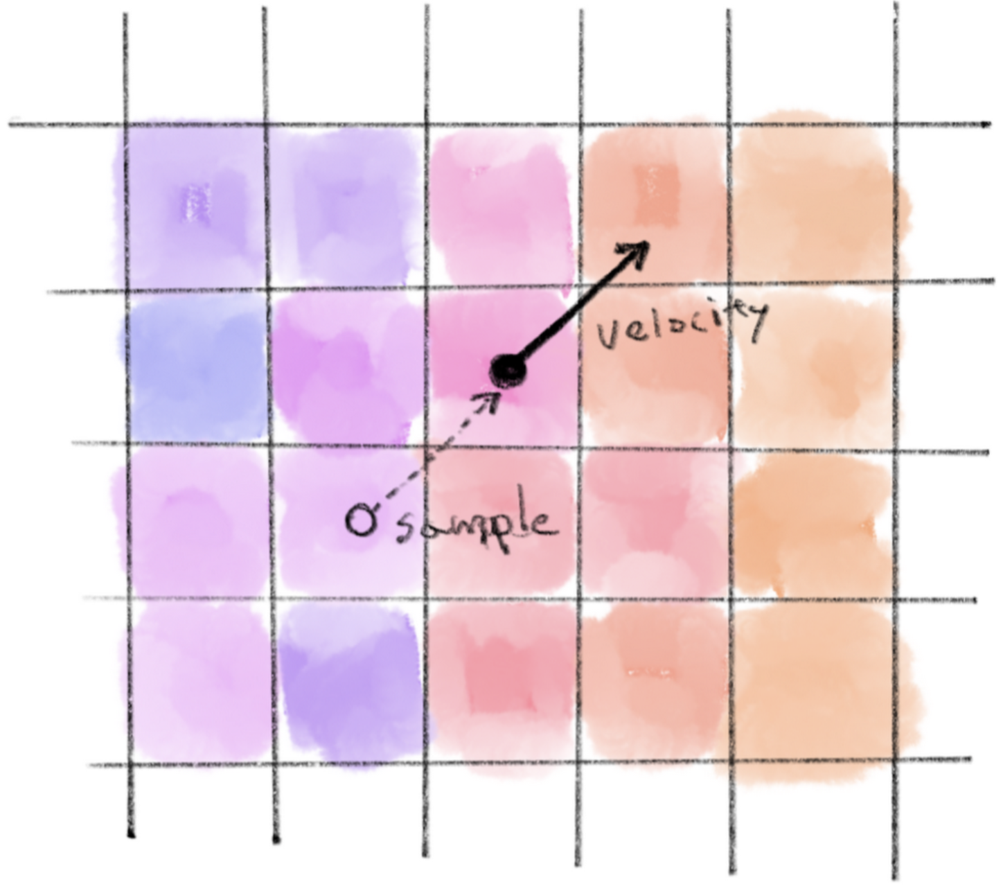
First, we will define the space as a grid of cells. We want to smoothly move paints, or different colors, around in this space. To do this, we will use two maps, specifically two 2D arrays, to capture the information for each cell. The color map stores the color values of each cell, while the velocity map stores a vector that represents the velocity, i.e. the information about the speed and direction of the water flow in each cell.

まず枡目（セル）が並んだグリッドとして空間を定義します。この空間で絵の具、または異なる色をスムーズに移動させるために、各セルの情報をキャプチャするための2つのマップ、具体的には2つの2D配列を使います。カラーマップは各セルの色の値を保持し、速度マップは速度、つまり各セルの水の流れの速さと向きを表すベクトルを格納します。

To move the colors, we will add the opposite vector of the velocity to the position of each cell and sample the color from that point. The idea is that the color at the sampled point will move to the position of the cell in the next frame. Typically, the sampling point is located in the middle of four cells, so we will interpolate the colors between these cells. Also, for this implementation, we assume that the top edge and the bottom edge, as well as the left edge and the right edge, are connected. This means that the sampling position will wrap around to the opposite side of the canvas if it goes out of bounds.

色を移動するためには、各セルの位置に速度のベクトルを逆にしたものを加え、その点から色をサンプリングします。ここではサンプリングした場所の色が、次のフレームでセルの位置に移動するものと考えています。たいていサンプリングする点は四つのセルの間になるので、セル間の色を補間して色を求めます。この実装では、上端と下端、左端と右端が繋がっていると仮定しています。つまり、サンプリング位置がキャンバスの外に出た場合は、反対側に折り返します。

// Update the colorMap based on the velocityMap
function updateColorMap() {
  const newColorMap = [];
  for (let y = 0; y < mapResolution; y++) {
    newColorMap.push([]);
    for (let x = 0; x < mapResolution; x++) {
      const sx = x - velocityMap[y][x][0];
      const sy = y - velocityMap[y][x][1];
			newColorMap[y].push(sampleMap(colorMap, sx, sy));
    } 
  }
  colorMap = newColorMap;
}

Take a look at our first step below. The arrows represent the velocity of each cell, and you will see the colors moving along these arrows. You can click on the canvas to restart the simulation. Try changing the initial condition in the initialize() function to see if you can make interesting patterns.

下のデモを見てください。矢印は各セルの速度を表し、その矢印に沿って色が移動していきます。キャンバスをクリックするとシミュレーションをリセットできます。initialize() 関数の中の初期条件を書きかえて面白いパターンが作れるか試してみましょう。

Advecting velocity

速度の流れ

This method is already useful and can create visually interesting effects if you experiment with the direction and magnitude of these velocities. In fact, this is essentially the same as what we observed on the Deformation and Feedback page. For example, you can deform and animate an image in various ways.

これだけでも、速度の向きや速さを変えて見た目に面白い効果を作り出せるので便利です。実際、これは変形とフィードバックのページで見たアイデアと本質的に同じもので、例えば画像を様々に変形したりアニメーションさせたりすることができます。

However, there are a few things missing to make it flow more realistically. One obvious thing is that the velocities are fixed in position. This is strange because, as water flows, the velocities should change according to the flow as well.

 しかし、よりリアルな流れを作るには、いくつかの足りない要素があります。まず目につくのは、速度が動かず固定されていることです。水が流れる時には速度も流れに応じて変化するはずなので、これは変です。

We can update the velocity map using the same method as how we moved the colors above. We sample the position of the cell minus the velocity vector to predict the velocity of the cell in the next frame.

速度マップの更新には、色を移動させるのと同じ方法が使えます。セルの位置から速度ベクトルを引いてサンプリングすることで、次のフレームでのセルの速度を予測します。

// Update the velocityMap based on the velocityMap itself
function updateVelocityMapAdvect() {
  const newVelocityMap = [];
  for (let y = 0; y < mapResolution; y++) {
    newVelocityMap.push([]);
    for (let x = 0; x < mapResolution; x++) {
      const sx = x - velocityMap[y][x][0];
      const sy = y - velocityMap[y][x][1];
      newVelocityMap[y].push(sampleMap(velocityMap, sx, sy));
    } 
  }
  velocityMap = newVelocityMap;
}

You can see this in action in the demo below.

下のデモで、実際の動きが見られます。

Navier-Stokes equations

ナビエ・ストークス方程式

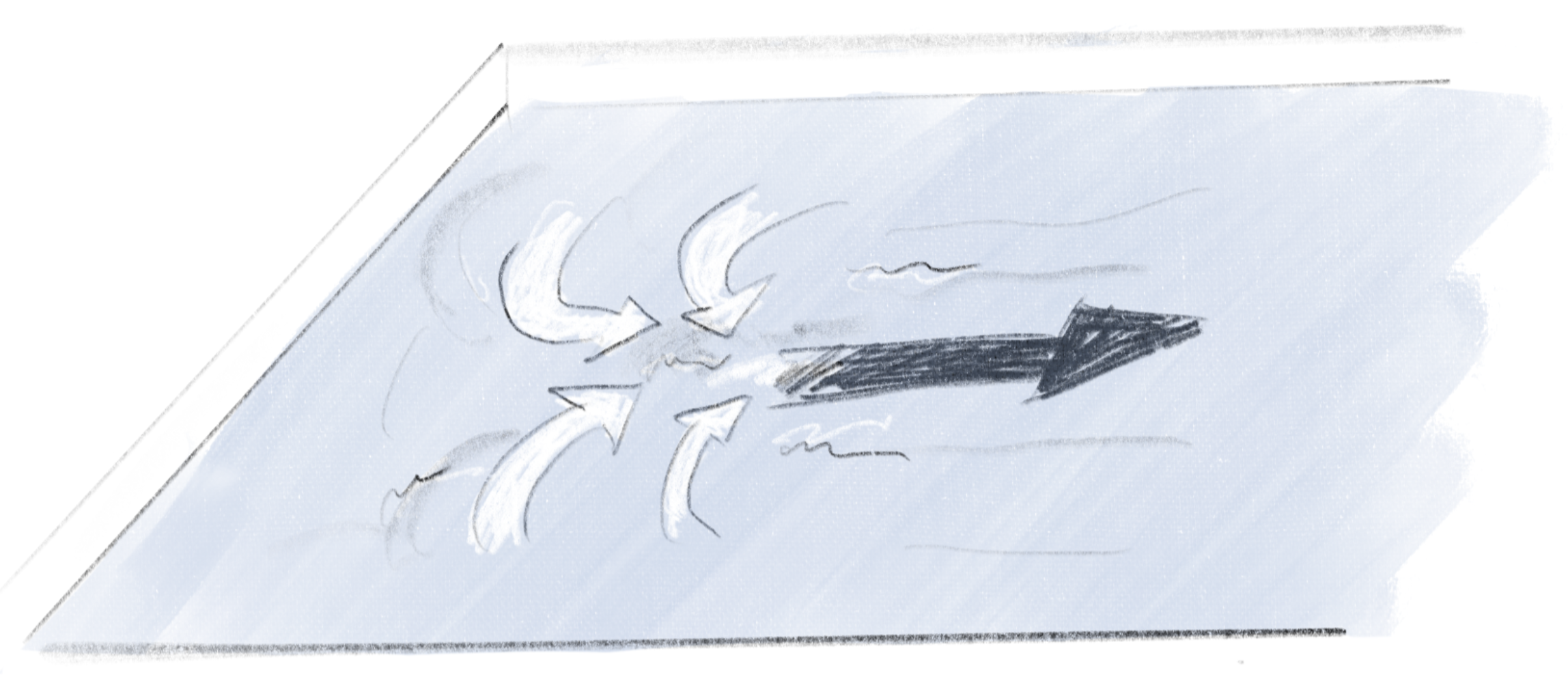
When you try to push water in a bathtub to the side, you will notice that the water immediately flows into the gap creating momentum. The water always seeks to maintain the same height on the surface. Also water is nearly incompressible. This means that if water is flowing out of a cell in a specific direction, an equivalent mass of water should be flowing into the cell from other directions.

バスタブの中で水を押すとすぐに水が隙間に流れ込み、水の動きが生まれるます。水は表面の高さ一定に保とうとします。また、水はほとんど圧縮することができません。このことを考えると、セルからある方向に水が流れ出せば、他の方向から同じ質量の水がセルに流れ込んでいくはずです。

In physics, this concept is expressed by following formulas called Navier-Stokes equations named after two physics scientists, Claude-Louis Navier and George Gabriel Stokes.

物理学では、この概念はナビエ・ストークス方程式と呼ばれる以下の式で表されます。この名前はクロード・ルイ・ナビエとジョージ・ガブリエル・ストークスという物理学者の名前に由来しています。

Continuity equation
連続の方程式

This equation represents the incompressibility of the fluid, ensuring it doesn’t accumulate or deplete at any point.

この式は流体が圧縮できないことを示していて、どの場所でも流体の量が増えたり減ったりしないことを保証しています。

$\begin{aligned} \nabla \cdot \mathbf{u} = 0 \end{aligned}$

Momentum equation
運動量の方程式

This equation is about the forces acting on the fluid and conservation of the momentum.

この式は、流体に作用する力と運動量の保存を表しています。

$\begin{aligned} \rho \left( \frac{\partial \mathbf{u}}{\partial t} + \mathbf{u} \cdot \nabla \mathbf{u} \right) = -\nabla p + \mu \nabla^2 \mathbf{u} + \mathbf{f} \end{aligned}$

Delegating the detailed explanation to the other site, let’s see what this means in practice in our implementation.

詳しい解説は他のサイトに任せるとして、これが実装にどう関わるのかを見てみましょう。

$u$ is the velocity, $\rho$(rho) is the density of the fluid, $p$ is the pressure. $\mu$(mu) is the viscosity of the fluid, and $f$ is an external force, but we ignore these two terms in our simulation (You can directly manipulate the velocity map if you want to apply extra forces.)

$u$は速度を表し、$\rho$は流体の密度、$p$は圧力を表します。$\mu$は流体の粘度、$f$は外から加わる力ですが、シミュレーションではこの2つの項は無視します（力を加えるには直接速度マップを操作することができます）。

These equations are really difficult to solve, and we don’t really have to. We will just approximate them numerically to get a good-looking result.

この方程式は非常に解くのが難しいのですが、実際に解く必要はありません。見た目に良いものができるよう数値的に近似すればOKです。

Divergence

発散

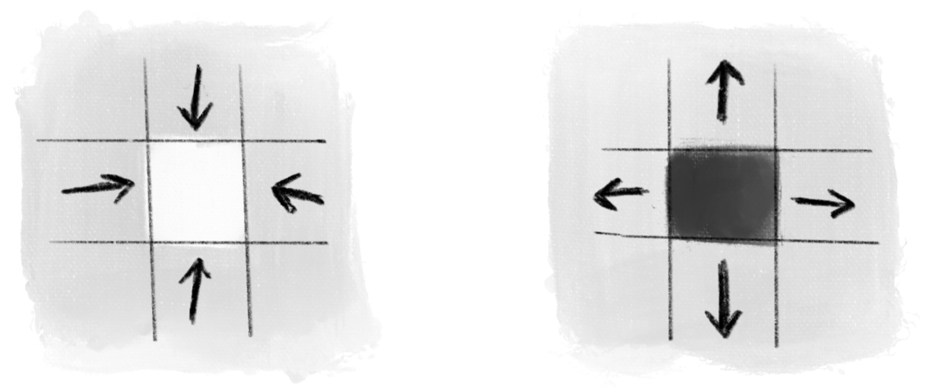
$\nabla \cdot \mathbf{u}$ is the divergence of the velocity. In this context, it represents the net amount of water flowing out of (or into) a given cell. This value is computed as the sum of the changes in velocity along the x-axis and y-axis, which can be approximated using numerical differentiation. Intuitively, if the arrows of the velocity point towards a cell, water is flowing in. If they point away, water is flowing out. The divergence measures the net effect by calculating the differences in these velocities. The equation $\nabla \cdot \mathbf{u} = 0$ is telling us that this divergence should be always zero. In reality, our simulation may not perfectly achieve this state, but we can approximate it. To adjust our velocity map, we first calculate the current divergences and store them in another map.

$\nabla \cdot \mathbf{u}$は速度の発散で、ここではあるセルから流れ出る（または流れ込む）水の総量を表します。この値は、x軸とy軸に沿った速度の変化の合計として計算されます。この変化は、数値微分を用いて近似することができます。直感的には、周りの速度の矢印がセルを指していれば水が流れ込んでいて、矢印がセルと逆を向いていれば流れ出していると考えられます。発散は、これらの速度の差を計算することで、その影響の合計を測定します。方程式 $\nabla \cdot \mathbf{u} = 0$ は、この発散が常にゼロになるべきだという主張です。現実のシミュレーションはこの状態を完全に達成するわけではありませんが、近似することはできます。速度マップを調整するために、まず現在の発散を計算し、別のマップに保存します。

// Update the divergenceMap based on the velocityMap
function updateDivergenceMap() {
  const newDivergenceMap = [];
  for (let y = 0; y < mapResolution; y++) {
    newDivergenceMap.push([]);
    for (let x = 0; x < mapResolution; x++) {
      const d = 
            velocityMap[y][wrap(x - 1)][0] - velocityMap[y][wrap(x + 1)][0] +
            velocityMap[wrap(y - 1)][x][1] - velocityMap[wrap(y + 1)][x][1];
      newDivergenceMap[y].push(d);
    } 
  }
  divergenceMap = newDivergenceMap;
}

In the demo below, the brighter the cells, the higher the divergence, and the darker the cell, the lower the divergence.

下のデモでは、セルが明るいほど発散の値が大きく、暗いほど低いことを示しています。

Pressure

圧力

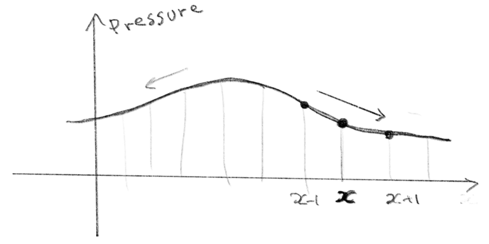
Next, we need to calculate the $p$ or the pressure that appears in the momentum equation to predict the next state of the velocity. I will skip the details again, but we can approximate the pressure based on the divergence above. A positive divergence means more water is entering, and a negative divergence means more water is leaving. We create another map for the pressure starting from all zeros, then apply the function below multiple times to “blur” the effect of the divergence.

続いて次の速度の状態を予測するために、運動量の式に現れる圧力 $p$を計算する必要があります。詳細は省略しますが、上記の発散に基づいて圧力を近似することができます。正の発散は水が流れ込むことを意味し、負の発散は水が出ることを意味します。圧力のための別のマップを作り全てのセルを0で初期化します。そして下の関数を繰り返し適用し、発散の影響を「ぼかし」ていきます。

Repeating this process is called the Jacobi method. It is basically making a first guess and refining it by making adjustments. This will help distribute the pressure well for the adjustment step below. Here, we only need a good enough result, and the demo applies the function only a few times per frame.

このプロセスの繰り返しはヤコビ法と呼ばれます。最初にまずざっくり予測を行い、繰り返し微調整することで精度を高めていきます。これにより、後の調整ステップで使うための圧力を適切に分散させることができます。デモではそれなりに良い結果が必要なだけなので、関数を毎フレーム数回だけ適用しています。

// Update the PressureMap
function updatePressureMap() {
  const newPressureMap = [];
  for (let y = 0; y < mapResolution; y++) {
    newPressureMap.push([]);
    for (let x = 0; x < mapResolution; x++) {
      const p = 0.25 * (divergenceMap[y][x]
      + pressureMap[y][wrap(x + 1)]
      + pressureMap[y][wrap(x - 1)]
      + pressureMap[wrap(y + 1)][x]
      + pressureMap[wrap(y - 1)][x]);
      newPressureMap[y].push(p);
    } 
  }
  pressureMap = newPressureMap;
}

Adjusting the velocity

速度を補正する

Now that we have the pressure, we can apply the momentum equation to adjust the velocity. Ignoring the viscosity and the external force, we can simplify the equation.

圧力が計算できたので運動量の式を適用して速度を調整できます。粘性と外力を無視して式を簡単にします。

$\begin{aligned} \rho \left( \frac{\partial \mathbf{u}}{\partial t} + \mathbf{u} \cdot \nabla \mathbf{u} \right) = -\nabla p \end{aligned}$

Dividing both sides by $\rho$ and rearranging to isolate $\begin{aligned} \frac{\partial \mathbf{u}}{\partial t} \end{aligned}$ , which represents the rate of the change of the velocity over time.

、$\begin{aligned} \frac{\partial \mathbf{u}}{\partial t} \end{aligned}$を取り出すために、$\rho$で両辺を割って並べ替えます。これは時間に対する速度の変化の割合を示します。

$\begin{aligned} \frac{\partial \mathbf{u}}{\partial t} = -\frac{1}{\rho} \nabla p - \mathbf{u} \cdot \nabla \mathbf{u} \end{aligned}$

$\nabla p$ and $\nabla \mathbf{u}$ are gradients, or vectors of derivatives along x and y axis, and we can approximate them numerically. The term $-\mathbf{u} \cdot \nabla \mathbf{u}$ represents the fact that velocities themselves moved around by the flow itself. This is already roughly taken care of the updateVelocityMapAdvect() function, so focusing only on $\begin{aligned} -\frac{1}{\rho} \nabla p \end{aligned}$:

$\nabla p$と$\nabla \mathbf{u}$は、勾配、つまりx軸とy軸に沿った微分のベクトルです。これは数値的に近似することができます。項$-\mathbf{u} \cdot \nabla \mathbf{u}$は、速度自体が流れによって移動することを表していますが、これはupdateVelocityMapAdvect()関数でカバーできているので、$\begin{aligned} -\frac{1}{\rho} \nabla p \end{aligned}$ にだけに注目します。

This term essentially represents the fact that water flows from areas of high pressure to areas of low pressure.

この項は基本的に、水は圧力の高い場所から低い場所へ流れることを表しています。

// Update the velocityMap integrating advaction and pressure

function updateVelocityMapIntegrate() {
  const newVelocityMap = [];
  for (let y = 0; y < mapResolution; y++) {
    newVelocityMap.push([]);
    for (let x = 0; x < mapResolution; x++) {
      const rho = 0.99;
			// Calculate the average pressure difference along x and y directions
			const pressure_diff_x = (pressureMap[y][wrap(x + 1)] - pressureMap[y][wrap(x - 1)]) / 2;
			const pressure_diff_y = (pressureMap[wrap(y + 1)][x] - pressureMap[wrap(y - 1)][x]) / 2;
			const fx = velocityMap[y][x][0] -  pressure_diff_x / rho;
			const fy = velocityMap[y][x][1] -  pressure_diff_y / rho;
      newVelocityMap[y].push([fx, fy]);
    } 
  }
  velocityMap = newVelocityMap;
}

$\nabla$ and $\nabla \cdot$ can be confusing because they look very similar. $\nabla$ is the gradient, which can tell you which way is uphill and steepness of the slope, while $\nabla \cdot$ represents the divergence, which is about if something is spreading out or coming together. If you are familiar with the dot product, you can make an association that $\nabla \cdot$ also yields a scalar value.
$\nabla$と$\nabla \cdot$はよく似ているので混乱しそうになります。$\nabla$は勾配で、どの方向が上りで、どれだけ傾斜しているかを示します。一方、$\nabla \cdot$は発散で、何かが散らばっていくのか集まってきているのかを教えてくれます。ドット積を知っていれば、$\nabla \cdot$も答えがスカラーになる点で似ていると覚えることができます。

The demo below puts everything together. Enjoy the nice and smooth swirl of the colors. rho = 0.99 is just an arbitrary number. Adjusting the value can make it look lighter or heavier. Try tweaking anything to see what happens.

下のデモはこれまでの全てを合わせたものです。美しく滑らかな色の渦を楽しみましょう。 rho = 0.99は適当な数値です。値を調整すると動きを軽くしたり、重くしたりすることができます。自由にコードをいじって、どんな変化が起こるか試してみましょう。

That’s it. We have covered all the basic concepts used in the GLSL version of the demo at the top. Take a look at the code and see if it makes sense. For GLSL shaders, please refer to the Book of Shaders (as always).

以上です。これで冒頭のGLSL版のデモで使われている基本的な概念は全てカバーしました。コードを見て、理解できるか試してください。GLSLシェーダーについては、（いつも通り）The book of shadersを参照してください。