Reaction-diffusion model 反応拡散モデル

Reaction-diffusion models are mathematical models used to describe the behavior and interplay of reactions and diffusion in various systems, such as in chemical and biological processes. They combine the effects of chemical reactions and diffusion to see how patterns change over time and space. Because these models can create complex patterns that are beyond imagination from simple rules, it is often used in the context of computer graphics and generative art as well.

反応拡散（Reaction-diffusion）モデルは、化学や生物学的なプロセスなど様々なシステムの振る舞いや、反応と拡散の相互作用を記述するために使われる数学モデルです。化学反応と拡散の効果を組み合わせて、パターンが時間と空間にわたってどのように変化するかを調べます。簡単なルールから思ってもみないような複雑なパターンを形成することができるので、コンピュータグラフィックスやジェネラティブアートの文脈でもよく用いられます。

Gray-Scott model

グレイスコットモデル

The Gray-Scott model is the most famous reaction-diffusion model. It was proposed by James P. Gray and Scott K. Scott in 1983. Since it is widely used, you may have encountered it before, to the point of becoming a cliché (so much so that I hesitated to add yet another article).

グレイ-スコットモデルは反応拡散の中でも最も有名なモデルです。1983年にジェームズ・P・グレーとスコット・K・スコットによって提案されました。このモデルは幅広く使い古されているので（わざわざここに書くか迷ったほどです）もしかすると、以前に見たことがあるかもしれません。

Before discussing the model in detail, let’s see what it looks like. Run the demo below. Did you see the black square spread, forming a clover-like shape, and eventually transforming into something that looks like a flower or worms? The Gray-Scott model is known for producing a variety of complex patterns depending on its parameters.

詳しくモデルを説明する前に、実際に見てみましょう。下のデモを実行してください。黒い四角形がクローバーのような形に広がり、やがて花か芋虫の群れにも見えるようなパターンに変化していくのが見られたでしょうか。グレイ・スコットモデルは、そのパラメータに応じてさまざまな複雑なパターンを生成することで知られています。

Break down of the model

モデルの概要

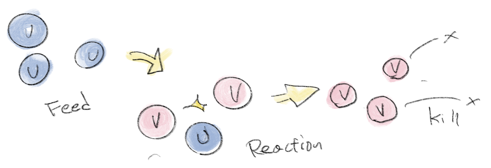
The Gray-Scott model is a model that describes the interaction and diffusion of two imaginary “substances”. It is like dropping two different chemicals into water and observing their reaction. Let’s call these substances as V and U. Several things happen simultaneously.

Diffusion: Just as ink dropped into a glass of water will spread out, substances U and V will also spread out over time.
Reaction: U and V react with each other. When they meet, U turns into V. The rate of the reaction depends on the concentrations of both substances.
Feed: We keep feeding U into the system to compensate for the amount lost during the reaction. The rate becomes faster when there is less U and slower when there is more.
Kill: We also get rid of excessive V. The rate is proportional to the amount of V.

グレイ・スコットモデルは、2つの架空の「物質」の相互作用と拡散を記述します。これは、水に異なる2つの化学物質を落としてその反応を観察するようなものです。これらの物質をVとUと呼びましょう。このモデルではいくつかのことが同時に起こります。

拡散: 水に落としたインクが広がるように、物質UとVも時間とともに広がります。
反応: UとVが触れると反応が起こり、UはV に変わります。反応の速度は両物質の濃度に依存します。
供給: 反応中に失われた U の量を補うために、システムには常にUが供給されます。Uが少ないと供給が速くなり、多いと遅くなります。
除去: システムから過剰なVを取り除きます。取り除く速さはVの量に比例します。

So, in short, both U and V gradually spread in the water, and when they meet, the reaction turns U into V. We keep feeding U and removing V to maintain the balance of the system and keep the dance of these substances interesting.

まとめると、UとVは徐々に水中に広がって行き、お互いが触れると反応が起こり、UがVに変わります。システムはUを供給しVを取り除いてバランスをとって、物質がダンスを続けるように保ちます。

The Gray-Scott model is expressed by the following formulas. Let’s decode them by converting them into executable code.

グレイ・スコットモデルは、以下の式で表されます。実行可能なコードに置き換えながら読み解いて行きましょう。

${\begin{aligned} \frac{\partial u}{\partial t} = Du \nabla ^2 u-uv^2 + f(1 - u) \end{aligned}}$

${\begin{aligned} \frac{\partial v}{\partial t} = Dv \nabla^2 v+uv^2 - v(f + k) \end{aligned}}$

To implement the Gray-Scott model, we will consider the space as a grid of cells. Each cell has two values, $u$ and $v$ , which represent the amount of substances U and V in the cell. The left side of the formulas ${\begin{aligned} \frac{\partial u}{\partial t} \end{aligned}}$ and ${\begin{aligned} \frac{\partial v}{\partial t} \end{aligned}}$ represent how much $u$ and $v$ change over a short time interval $\partial t$ .

グレイ-スコットモデルを実装するために、空間をセルのグリッドとして考えます。セルごとの物質UとVの量を $u$ と $v$ とします。式の左側の ${\begin{aligned} \frac{\partial u}{\partial t} \end{aligned}}$ と ${\begin{aligned} \frac{\partial v}{\partial t} \end{aligned}}$ は、 $u$ と $v$ が短い時間 $\partial t$ の間にどれだけ変化するかを表しています。

Diffusion

拡散

The terms $Du \nabla^2 u$ and $Dv \nabla^2 v$ model the diffusion of U and V, i.e., how they spread over time. $Du$ and $Dv$ are constants, the diffusion rates for $u$ and $v$ respectively.

$Du \nabla^2 u$ と $Dv \nabla^2 v$ の項は、UとVの拡散、つまり時間の経過とともにどのように広がるかをモデル化しています。 $Du$ と $Dv$ は、それぞれ $u$ と $v$ の拡散率を表す定数です。

We saw this formula for diffusion on the diffusion page.

下は拡散のページで触れた拡散の式です。

${\displaystyle {\begin{aligned} \frac{\partial u}{\partial t} = \alpha \frac{\partial^2 u}{\partial x^2} \end{aligned}}}$

You can think of $Du$ and $Dv$ as $\alpha$ in this equation. $\nabla^2$ is called Laplacian operator, and in this context it represents the sum of diffusion across multiple dimensions. Since we are working in 2D, we can say:

$Du$ と $D v$ は上の式の $\alpha$ に相当すると考えられます。 $\nabla^2$ はラプラシアンオペレーターと呼ばれ、この場合は複数の次元をまたいだ拡散の合計を表します。これは2Dの場合このように書けます。

${\begin{aligned} \nabla^2 u = (\frac{\partial^2 u}{\partial x^2} + \frac{\partial^2 u}{\partial y^2})\end{aligned}}$

and using numeric approximation this becomes:

これを数値的に近似をすると下のコードになります。

const leftU = u[wrap(i - 1, N_GRIDS)][j];
const rightU = u[wrap(i + 1, N_GRIDS)][j];
const upU = u[i][wrap(j - 1, N_GRIDS)];
const downU = u[i][wrap(j + 1, N_GRIDS)];
laplacian_u[i][j] = (leftU + rightU + upU + downU - 4 * u[i][j]) / (dx * dx);
...
let dudt = Du * laplacian_u[i]...

Basically, this calculates the diffusion using the value of the current cell and its four neighboring cells. The wrap function is used to wrap the sides of the grid to the other end. The same goes for V as well but $Du$ is typically larger than $Dv$ . It is crucial for U and V to spread at different rates in order to generate interesting patterns.

これは現在のセルの値とその隣接する4つのセルを使って拡散を計算します。wrap関数は、グリッドの側面を他の端に回り込ませるためのものです。Vも同様に書けますが、面白いパターンが生まれるためにはUとVが異なる速度で広がることが大事なので大抵は $D u$ に $D v$ より大きい値を用います。

Reaction

反応

The term $uv^2$ models the reaction where U reacts with V and turn into V. The translation to code is just straightforward: u[i][j] * v[i][j] * v[i][j]. Because U becomes V, we subtract the value from U and add the same amount to V.

$uv^2$ の項は、UがVと反応してVに変わる様子をモデル化しています。コードへの変換は式そのままu[i][j] * v[i][j] * v[i][j]となります。UがVに変わるので、Uから値を引き、同じ量をVに加えます。

let dudt = Du * laplacian_u[i] - u[i][j] * v[i][j] * v[i][j]...

let dvdt = Dv * laplacian_v[i] - u[i][j] * v[i][j] * v[i][j]...

Feed and kill

供給と除去

The expression $f(1 - u)$ represents the feed rate of $u$ , while the term $v(f+k)$ represents the death rate or kill rate for $v$ . In this context, $f$ and $k$ are constants. You can see that the feed rate decreases as $u$ decreases, and the kill rate increases proportionally to $v$ . The fact that $f$ appears in both equations reflects an underlying symmetry or interdependence in the model between the two substances U and V, and these terms maintain the balance of the system, ensuring that both “U” and “V” are always present.

$f(1 - u)$ は $u$ の供給率を表し、 $v(f+k)$ は $v$ の除去率を表します。ここでは $f$ と $k$ は定数です。 $u$ が減少するにつれて供給率は減り、 $v$ に比例して除去率が増えることがわかります。両方の式に $f$ が現れるのは、モデル内の物質UとVの間の基本的な対称性や相互依存性があることを表していて、これら項はシステムのバランスを維持し、常にUとVが存在することを保証する働きをします。

let dudt = Du * laplacian_u[i][j] - ... + f * (1.0 - u[i][j]);

let dvdt = Dv * laplacian_v[i][j] + ... - (f + k) * v[i][j];

Shader simulation

シェーダーによるシミュレーション

Let’s see the Gray-Scott model in action in much larger scale. Different from the demo above, this one is implemented using a GLSL shader. The Gray-Scott model can become computationally heavy as it processes all the cells every frame, but we can parallelize this process by using a shader. Experiment with different constants and observe how the pattern changes.

より大きなスケールでグレイスコットモデルを見てみましょう。ここまでとは異なり、このデモはGLSLシェーダーを使って実装されています。グレイスコットモデルは、すべてのセルをフレームごとに処理するので計算が重くなりますが、シェーダーを使うとプロセスを並列化することができます。異なる定数の値を試して、パターンがどのように変化するか観察しましょう。

float dx = 0.1; // Distance per pixel in simulation space
float dt = 1.0; // Time increment per frame
float Du = 0.002; // Diffusion rate for U chemical
float Dv = 0.001; // Diffusion rate for V chemical
float f = 0.022, k = 0.051; // Feed and kill rates for the reaction

To learn about shaders, please read The Book of Shaders.
シェーダーについては、The Book of Shadersを読んでください。

The Gray Scott model is just one example of reaction-diffusion models. You can look for more examples, or it can be even more enjoyable to create your own. Reaction-diffusion models were originally designed for studying chemical reactions, but for the purpose of sketching, your model doesn’t have to be accurate or resemble anything in the real world. Feel free to modify the formula, add new terms and logic, and see what happens. It might be fun to add more than two different kinds of chemicals. I’m not sure if the following examples strictly qualify as reaction-diffusion models (probably not), but they are largely inspired by the idea of simulating reactions between substances and use similar logic.

グレイ・スコットモデルは、反応拡散モデルのひとつの例です。他の例を探しても良いですし、自分自身で作成する方がもっと楽しいかもしれません。反応拡散モデルはもともと化学反応の研究のために考えだされましたが、スケッチに使う分にはモデルが正確であったり、現実世界の何かに似ている必要もありません。式を自由に変更し、新しい項やロジックを追加してどうなるかを見てみましょう。科学物質の種類を3つ以上に増やしても面白いかもしれません。以下の例は厳密に反応拡散モデルに該当するかはわかりませんが（多分違う）、物質間の反応をシミュレートするというアイデアに基づいて似たようなロジックを使っています。