Other Key Layers その他の重要なレイヤー

Let’s examine the other key layers we haven’t discussed yet.

まだ詳しく議論していない、その他の重要なレイヤーを見ていきましょう。

Positional Encoding

位置エンコーディング

Since our model contains no recurrence and no convolution, in order for the model to make use of the order of the sequence, we must inject some information about the relative or absolute position of the tokens in the sequence. To this end, we add “positional encodings” to the input embeddings at the bottoms of the encoder and decoder stacks.

本モデルは再帰や畳み込みを含まないため、シーケンスの順序を利用するには、トークンの相対的または絶対的な位置に関する情報を挿入する必要がある。その目的のため、我々はエンコーダとデコーダのスタックの最下部において、入力の埋め込み（Embedding）に「位置エンコーディング（Positional Encodings）」を加算する。

The attention mechanism can process relationships between all embeddings at once. However, the attention layer itself has no way to distinguish tokens based on their position in the sentence. This is a significant problem since word order is critical information.

アテンション機構は、すべての埋め込み間の関係を一度に処理できます。しかし、アテンション層自体には、文中の位置に基づいてトークンを区別する方法がありません。単語の順序は非常に重要な情報なのでこれは大きな問題です。

To solve this, positional encoding layers at the start of the encoder and decoder add position information to each token. Think of this as a timestamp for each token. The authors use sine and cosine functions at different frequencies to create these timestamps.

これを解決するため、エンコーダとデコーダの開始部にある位置エンコーディング層が、それぞれのトークンに位置情報を追加します。これはトークンに対するタイムスタンプのようなものだと考えてください。論文では、異なる周波数のサイン関数とコサイン関数を使用して、これらのタイムスタンプを作成しています。

$PE_{(pos, 2i)} = \sin(pos / 10000^{2i/d_{model}})$

$PE_{(pos, 2i+1)} = \cos(pos / 10000^{2i/d_{model}})$

$pos$: The position of the word in the sentence (0 for $\text{I}$, 1 for $\text{_ate}$, etc.).

$i$: The dimension index (from 0 to 511).

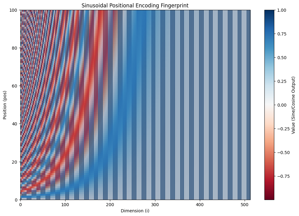
The result is a 512-dimensional vector of numbers between −1 and 1. And the layer simply adds this vector to the embeddings for each token.

結果は−1から1の間の数値からなる512次元のベクトルになります。この層は、それぞれのトークンの埋め込みに対して単純にこのベクトルを加算します。

Let’s visualize this with code. Below are the maps of the output from this formula at different zoom level.

コードを使ってこれを可視化してみましょう。下は、この数式の出力を異なるズームレベルで表示したものです。

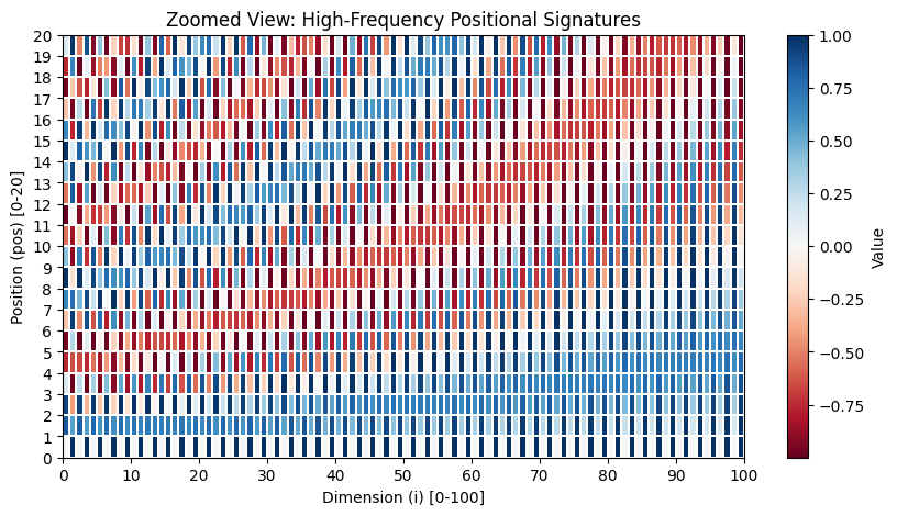
Can you see that every row (position) has a unique combination of values across the 512 dimensions? Even if the same token $\text{_apple}$ appears at position 3 and position 50, the added stamp will make them different.

すべての行（位置）が512次元全体にわたって一意な値の組み合わせになっていることがわかるでしょうか。たとえ同じトークン$\text{_apple}$が位置3と位置50に現れたとしても、加算されたスタンプによってそれらは異なるものになります。

we hypothesized it would allow the model to easily learn to attend by relative positions, since for any fixed offset $k$, $PE_{pos+k}$ can be represented as a linear function of
$PE_{pos}$.

我々は、いかなる固定されたオフセット $k$ に対しても $PE_{pos+k}$ が $PE_{pos}$ の線形関数として表現できることから、この手法（サイン・コサイン関数）を用いることで、モデルが相対的な位置に基づいたアテンションを容易に学習できるようになると仮定した。

The authors chose this specifically because $PE_{pos+k}$ can be represented as a linear function of $PE_{pos}$. This means the model can mathematically “calculate” the distance between any two words simply by comparing their encodings.

著者らがこれを選択したのは、$PE_{pos+k}$が$PE_{pos}$の線形関数として表現できるという理由からです。これにより、モデルはエンコーディングを比較するだけで、任意の2つの単語間の距離を数学的に「計算」することができます。

If you’re wondering why this is linear, notice that moving from one position to another is a rotation in high dimensional space, and rotations can be expressed as matrix multiplications.

なぜこれが線形なのか不思議に思えるなら、ある位置から別の位置への移動は高次元空間における回転であり、回転は行列の乗算として表現できることに注目しましょう。

The main encoder and decoder components have no built-in notion of position or order. They can’t even see the original embeddings and positional encodings separately since these are added together before processing. Only through training does the model learn to adjust its internal parameters to act as if it understands both the words and their positions.

メインのエンコーダとデコーダのコンポーネントには、位置や順序の概念が組み込まれていません。元の埋め込みと位置エンコーディングは処理前に加算されるため、それらを個別に見ることすらできません。訓練を通じてのみ、モデルが単語とその位置の両方を理解しているかのように振る舞うよう、内部パラメータが調整されるのです。

Linear and Softmax

線形層とソフトマックス

The final part of the architecture consists of linear and softmax layers. These layers generate the output—a probability for each token in the vocabulary. The linear layer is the key component here, as the softmax simply normalizes its output.

アーキテクチャの最後の部分は、線形層とソフトマックス層で構成されています。これらの層はボキャブラリに含まれるそれぞれのトークンに対する確率を出力として生成します。ソフトマックスは単に出力を正規化するだけなので、線形層がここでの主要な役割を果たします。

The linear layer takes only the last vector from the decoder’s output. This is the last token of the previously generated text, but it’s loaded with all the useful context from the original input and preceding output.

線形層は、デコーダーの出力から最後のベクトルのみを受け取ります。これは以前に生成されたテキストの最後のトークンですが、元の入力と先行する出力からの有用なコンテキストがすべて込められています。

This is only metaphorically true. More precisely, it’s a vector that, when fed into the linear layer, produces the correct output. Since all parameters in the model are trained together, the outputs between layers only make sense within the context of those specific layers. A human would find it very difficult to understand what this vector means by looking at it directly (though if we examine it closely, we can expect to find interesting geometric relationships—for example, vectors that yield similar results are probably close together in the space).

これは比喩的な表現で、より正確には、線形層に入力されたときに正しい出力を生成するベクトルといえます。モデル内のすべてのパラメータは一緒に訓練されるため、層の間の出力はその特定の層の文脈内でのみ意味を持ちます。人間がこのベクトルを直接見てその意味を理解することは非常に困難です。（とはいえ詳しく調べれば興味深い幾何学的関係が見つかるはずで、例えば、似た結果を生み出すベクトルは空間内で互いに近くに配置されているでしょう。）

The paper doesn’t mention the details of this layer, but it’s a simple fully connected (dense) layer.

論文ではこの層の詳細には触れられていませんが、単純な全結合層です。

$\text{Output} = xW + b$

This maps the final 512-dimensional vector from the top of the decoder stack ($x$) to a vector the size of the entire vocabulary.

これは、デコーダスタックの最上部からの最終的な512次元ベクトル（$x$）を、ボキャブラリ全体のサイズのベクトルにマッピングします。

$W$ is the Weight Matrix. In the base model, this matrix is $512 \times V$ (where $V$ is the vocabulary size). Every single token in the dictionary has its own 512-dimensional set of weights in this matrix. $b$ is The Bias Vector. This is a $V$-dimensional vector added to the result.

$W$は重み行列です。基本モデルでは、この行列は$512 \times V$（$V$はボキャブラリサイズ）です。辞書内のすべてのトークンは、この行列内に独自の512次元の重みのセットを持っています。$b$はバイアスベクトルです。これは結果に加算される$V$次元のベクトルです。

The Linear layer gives us raw numbers that can be anything from negative infinity to positive infinity. The Softmax layer squashes them into a probability distribution where every number is between 0 and 1, and they all sum to 100%.

線形層は負の無限大から正の無限大まで、任意の値を取りうる生の数値を出力します。ソフトマックス層はそれらを0から1の間の値に変換し、すべての合計が100%になる確率分布を作ります。

$\displaystyle{ \text{softmax}(z_i) = \frac{e^{z_i}}{\sum_{j=1}^{K} e^{z_j}} }$

The demo below shows how the softmax function works.

下のデモは、ソフトマックス関数がどのように機能するかを示しています。

The model then chooses the token with the highest probability, feeds it back into the bottom of the decoder, and repeats the process until it generates an $\text{<EOS>}$ (End of Sentence) token.

モデルは最も高い確率を持つトークンを選択し、それをデコーダの最下部に入力し、$\text{<EOS>}$（文末）トークンを生成するまでこのプロセスを繰り返します。

Next

On the next page, we’ll discuss the conclusion part of the paper and the application of the architecture to wrap up the series.

次のページでは、論文の結論部分とアーキテクチャの応用について議論し、シリーズを締めくくります。

Conclusions and Applications 結論と応用