Convolution コンボリューション
Convolution is an operation used in image processing and machine learning that is performed by applying a filter or a kernel to the source data, in the case of an image, an array of pixels. Convolution is used in blurring, sharpening, edge detection and many other image processing tasks. Let’s look at a practical example.
コンボリューション(畳み込み)は、画像処理やマシンラーニングで用いられる演算で、フィルタ(カーネル)を元になるデータ、画像の場合はピクセルの配列に適用することで実行されます。コンボリューションはぼかし、シャープ、エッジ検出など、画像処理で幅広く使用されます。実際の例を見てみましょう。
Blur
ぼかし
First, let’s take a look at a demo. On the left is an image of a black circle, and on the right you can see how a filter is applied to blur the same image.
まずはデモを見てみましょう。左には黒い丸の画像があり、右では同じ画像にフィルターをかけてぼかしていく様子が見られます。
On a computer, an image is just a sequence of numbers. If black is 0 and white is 1, the table below is an image of a white square on a black background.
コンピュータ上では画像はただの数列です。黒を0、白を1とすると下の表は黒い背景に白い正方形が描かれた画像になります。
| 0 | 0 | 0 | 0 | 0 |
| 0 | 1 | 1 | 1 | 0 |
| 0 | 1 | 1 | 1 | 0 |
| 0 | 1 | 1 | 1 | 0 |
| 0 | 0 | 0 | 0 | 0 |
A filter is also defined as an array. This is the array used in the demo.
フィルターも配列として定義します。 これがデモで使った配列です。
| 0.1 | 0.1 | 0.1 |
| 0.1 | 0.2 | 0.1 |
| 0.1 | 0.1 | 0.1 |
We select one pixel from the image, let’s say the second from the left and the second from the top. We take the surrounding pixels as well and multiply them with the filter.
画像からピクセルをひとつ選びます。ここでは左から2番目、上から2番目のピクセルにします。周囲のピクセルも取り出し、フィルターと掛け合わせます。
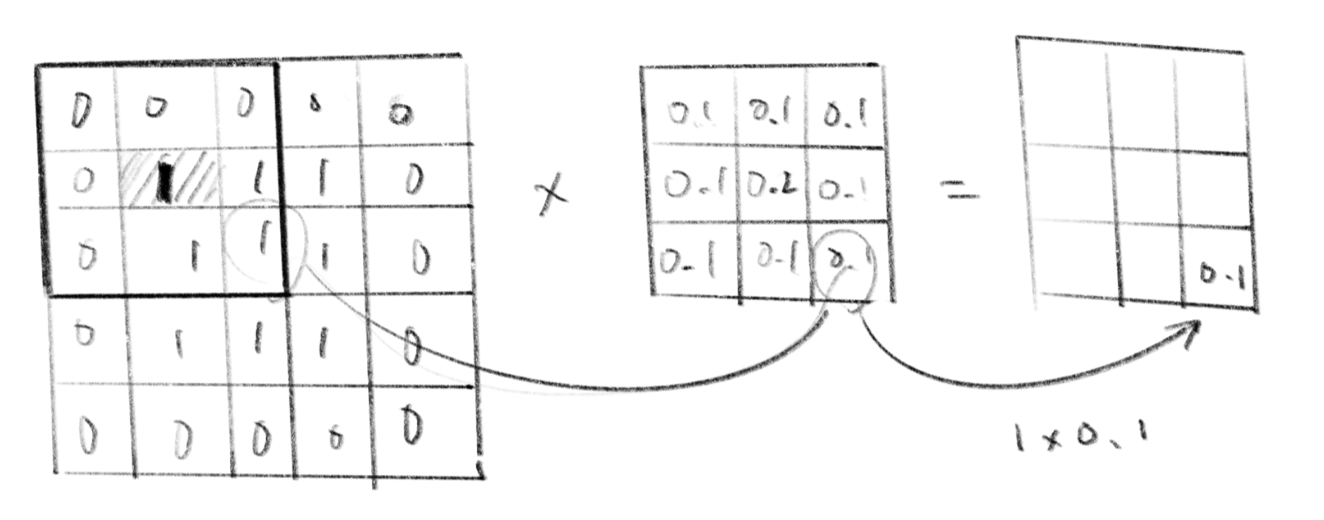
And we get an array like this.
こんな配列が得られます。
| 0 | 0 | 0 |
| 0 | 0.2 | 0.1 |
| 0 | 0.1 | 0.1 |
We add all these numbers together () and replace the original pixel with the sum.
この数値を全て足し合わせ()、元のピクセルを置き換えます。
| 0 | 0 | 0 | 0 | 0 |
| 0 | 0.5 | 1 | 1 | 0 |
| 0 | 1 | 1 | 1 | 0 |
| 0 | 1 | 1 | 1 | 0 |
| 0 | 0 | 0 | 0 | 0 |
If you see these arrays as vectors, multiplying corresponding components and adding them all together makes their dot product.
これらの数列をベクトルと考えると、対応する成分を掛け合わせ、すべてを足し合わせた結果は内積となります。
Let’s repeat the same for all pixels. We assume 0 for the values where the filter extends beyond the image. The result looks like this.
同じ作業を全てのピクセルに対して行います。フィルターが画像からはみ出る部分の値は0として計算します。こんな結果になります。
| 0.1 | 0.2 | 0.3 | 0.2 | 0.1 |
| 0.2 | 0.5 | 0.7 | 0.5 | 0.2 |
| 0.3 | 0.7 | 1 | 0.7 | 0.3 |
| 0.2 | 0.5 | 0.7 | 0.5 | 0.2 |
| 0.1 | 0.2 | 0.3 | 0.2 | 0.1 |
Can you see how this array looks like a blurred version of the original square if you think of the values as the brightness of gray? Take another look at the demo with this in mind, and you will have a better idea of what is happening.
値をグレーの明るさだと考えるとこの配列は元の正方形をぼかしたように見えるのがわかるでしょうか。これを踏まえてもう一度デモを見ると何が起こっているのかよくわかるでしょう。
A filter can be any size. The demo below shows an example of a 7 x 7 filter with a normal (Gaussian) distribution for its values. This is called Gaussian Blur.
フィルタの大きさは自由に決めることができます。下のデモは7×7のフィルタの値に正規分布(ガウス分布)を用いた例です。これはガウシアンブラー、またはガウスぼかしなどと呼ばれます。
Mathematically, convolution is defined with the following formula as the integral of the product of the two functions after one is reflected about the y-axis and shifted (Wikipedia). We will only cover discrete convolutions used in image processing, but please look it up if you are interested. The blurring effect above can be thought of as a discrete pixel approximation of what is better thought of as a continuous function in optics.
数学的には、コンボリューションは2つの関数の一方をy軸について反射させ、シフトさせた後の積の積分として下の式で定義されます(Wikipedia)。ここでは離散的なコンボリューションだけを扱いますが、興味がある方は調べてみましょう。上のぼかしの処理は、光学的には連続的な関数として考えた方が良いものを離散的なピクセルで近似したものと考えることができます。
Edge Detection
エッジ検出
Laplacian
ラプラシアン
The filter below can be used to extract the edges from an image. Consider specific image values to understand how it works.
下のようなフィルタを用いると画像の輪郭部分を取り出すことができます。働きを理解するには具体的な画像の値を当てはめて考えてみましょう。
| 0 | -1 | 0 |
| -1 | 4 | -1 |
| 0 | -1 | 0 |
This operation is called the Laplacian and is actually the calculation of the second-order derivative, or the change of change, which also appeared in the wave equation. Let’s name the pixel of interest and its surrounding pixels.
この操作はラプラシアンと呼ばれ実は波動方程式でも登場した2階微分、つまり変化量の変化量を求める計算になっています。注目するピクセルとその周りのピクセルに名前を付けます。
| p0,−1 | ||
| p−1,0 | p0,0 | p1,0 |
| p0,1 |
(a) The change of change along the x-axis
x軸に沿った変化量の変化量
(b) The change of change along the y-axis
y軸に沿った変化量の変化量
The filter below can be used to detect diagonal changes as well. This is also a Laplacian filter.
下のフィルタを使うと斜め方向の変化も検知できます。これもラプラシアンフィルタです。
| -1 | -1 | -1 |
| -1 | 8 | -1 |
| -1 | -1 | -1 |
Sobel/Prewitt
ソーベル/プレヴィット
Other commonly used filters include Sobel and Prewitt, which are first-order derivatives. Since these filters are directional, they need to be applied separately for the vertical and horizontal directions. The table below shows Sobel on the left and Prewitt on the right. The demo displays the absolute value of the result after applying the Sobel filter.
他によく使われるものにはソーベルやプレヴィットといったフィルタがあって、これは一階の微分になります。方向性があるので垂直方向と水平方向に分けて繰り返す必要があります。下の表の左がソーベル、右がプレヴィットです。デモではソーベルフィルタをかけた結果の絶対値を表示しています。
| -1 | 0 | 1 |
| -2 | 0 | 2 |
| -1 | 0 | 1 |
| -1 | 0 | 1 |
| -1 | 0 | 1 |
| -1 | 0 | 1 |
Sharpen
シャープ
Next, let’s look at a filter for sharpening, or emphasizing, the edges of an image.
次はシャープ、つまり画像のエッジを際立たせる効果を持ったフィルターを見てみましょう。
Laplacian
ラプラシアン
The Laplacian filter used in edge detection can also be used to sharpen an image. As shown below, we can use a filter with smaller values then add the result to the original image.
エッジ検知でも使ったラプラシアンフィルタは画像をシャープにするためにも使えます。下のように少し値を小さめにしたフィルタをかけて、得た値を元の画像に足してやります。
| -0.2 | -0.2 | -0.2 |
| -0.2 | 1.6 | -0.2 |
| -0.2 | -0.2 | -0.2 |
Unsharp Mask
アンシャープマスク
One of the more commonly used methods is unsharp masking. It is a bit odd to call it “un”-sharp when it actually sharpens the image, but this seems to be derived from the fact that a blurred version of the image is used in the process.
より一般的に使われる方法のひとつにアンシャープマスクがあります。画像をシャープにするのに「アン」シャープと呼ばれるのはちょっと変ですが、これは元画像をぼかしたものを処理に用いることから来ているようです。
To apply an unsharp mask, we calculate the difference between the blurred image and the original image, and subtract the difference from the original image. This sounds a little confusing, but we can write it in a simple formula as follows, where is the value of the original image and is the value of the blurred image.
アンシャープマスクをかけるにはぼかした画像とと元画像との差分を求め、さらにその差分を元の画像から引いてやります。文章だと分かりにくいですが、を元画像の値、をぼかした後の画像の値とすると下記のようなシンプルな式になります。
This technique is more flexible than the Laplacian filter because you can choose different types and sizes of the blur filter as you want. A 3x3 Gaussian blur is used in the demo below.
この手法では好きなぼかしのフィルタや大きさを選べるのでラプラシアンよりも自由度があります。下のデモでは3x3のガウシアンブラーを用いています。
Make your own filters
試してみよう
We have covered some of the most commonly used filters, but of course, you can create convolutions in any way you like. Before running the demos below, try guessing what kinds of effects these filters will have. You can also experiment with creating your own filters using different sizes, values, and images.
よく使われるフィルタをいくつか見てきましたが、もちろんコンボリューションは自分の好きなように作ることができます。下のフィルタにはどんな効果があるでしょうか。デモを走らせる前に考えてみましょう。フィルタの大きさや値、画像を変えていろいろ試してみましょう。
| 0 | 0 | 0 |
| 0 | 0 | 1 |
| 0 | 0 | 0 |
| 0 | 1 | 0 |
| 1 | 1 | 1 |
| 0 | 1 | 0 |