Fractal フラクタル

A fractal is a pattern or shape that repeats the same structure at different scales, in such a way that a part of the shape resembles the whole, and a sub-part of a part resembles the larger part.

フラクタルは、部分が全体に似ていたり、またその一部がより大きな部分に似ていたりと、異なるスケールで同じ構造を繰り返すパターンまたは形状です。

This property, called self-similarity, is key to modeling many complex structures and patterns found in nature, such as coastlines, mountains, clouds, and tree branches. Objects and lives in nature often form fractal-like structures in the process of building themselves, where similar patterns recur at progressively smaller or larger scales. Understanding this principle can help us sketch them.

この性質は自己相似性と呼ばれ、海岸線や、山、雲、木の枝など、自然に見られる多くの複雑な構造やパターンをモデリングするため重要な概念です。自然界の物体や生命は、自己を構築する過程でしばしば、同様のパターンがより小さな、または大きなスケールで繰り返し現れる、フラクタルのような構造を形成します。この原理を理解することは、これらの現象をスケッチする役に立ちます。

There seems to be a case where the demos on this page don’t load properly when you open multiple ones. If this happens, try hitting the Rerun button on the bottom right, or the arrow button on the top right to open it in a new window.
このページのデモを複数開いた時にうまくロードされない場合があるようです。その場合は右下のRerunボタンを押すか、右上の矢印ボタンを押して新しいウィンドウで開いてみてください。

Mandelbrot set and Julia set マンデルブロ集合とジュリア集合

The Mandelbrot set and Julia set are two of the most famous fractals in mathematics. If you take a book about fractal, there is a good chance that the cover features either or both of them.

マンデルブロ集合とジュリア集合は、数学で扱うフラクタルの中でも最も有名ものです。フラクタルについての本の表紙には大抵このどちらか、または両方があしらわれています。

They are closely related to teach other and defined by the behaviors of complex functions under infinite iteration. But setting the math aside for now, let’s take a look at them and observe how they have infinite details resembling itself, no matter how much we zoom in.

これら2つの集合は密接に関連しており、複素関数の無限反復による振る舞いで定義されます。しかし、数学は一旦脇に置いて、これらの集合がどれだけズームインしても、自分自身に似た形を持つ無限のディティールを持っていることを観察しましょう。

Sierpiński Carpet シェルピンスキーカーペット

Let’s look at a much simpler example of fractal. The demo below draws a pattern called Sierpiński Carpet. This is a great starting point, because not only is it easier to understand, but it represents the concept of self-similarity more directly than the Mandelbrot set or Julia set do.

はるかに単純なフラクタルの例を見てみましょう。以下のデモは、シェルピンスキーカーペットと呼ばれるパターンを描きます。これは素晴らしい出発点です、なぜならそれは理解しやすいだけでなく、マンデルブロ集合やジュリア集合よりも自己相似性の概念を直接的に表現します。

Sierpiński Carpet can be made by following the steps below infinitely.

シェルピンスキーカーペットは、以下の手順を無限に続けることで作成できます。

1. Start from a square. 正方形から始めます。

2. Divide the square into a 3x3 grid of smaller squares. 正方形を3x3のグリッドに分割します。

3. Remove the tile in the center, leaving 8 smaller squares around the perimeter. 中央のタイルを取り除き、周囲に8つの小さな正方形が残るようにします。

4. For all the remaining tiles, go back to the step 2 and repeat the process. ステップ2に戻り、残るすべてのタイルに対して同じプロセスを繰り返します。

The demo below renders the Sierpiński Carpet. Can you see how each square repeats the same structure inside, scaling down recursively? The demo below renders the Sierpiński Carpet. In reality, we cannot repeat the process infinitely, so it only applies several iterations, then reverts back to the initial state.

以下のデモでは、シェルピンスキーカーペットを描画します。それぞれの正方形が同じ構造を持ちながら再帰的に縮小し続ける様子を確認できるでしょう。現実ではプロセスを無限に繰り返すことは不可能なので、デモは数回のプロセスを繰り返した後、初期状態に戻ります。

Instead of removing the center piece, we can remove any one piece from each 3x3 grid and repeat that indefinitely. The result is still a fractal shape with the exact same Hausdorff dimension, which we will cover in a section below. The randomness can add an organic feel to it, resembling a natural sponge or a grain texture on a rock.

中心のピースを取り除く代わりに、3x3のグリッドからランダムに1つピースを取り除き、そのプロセスを無限に繰り返すこともできます。結果はまったく同じハウスドルフ次元（これについては後のセクションで説明します）を持つフラクタル形状となります。ランダムにすることで有機的な感じが加わり、天然のスポンジ（海綿）や岩の粒子などのテクスチャに似た表情になりました。

Koch Curve コッホ曲線

The Koch curve is another example of a simple fractal shape that can be drawn by following the steps below.

コッホ曲線は、別のシンプルなフラクタル形状の例で、以下の手順に従って描くことができます。

1. Start with a straight line segment. 線分から始めます。

2. Divide the line segment into three equal parts. 線分を3等分します。

3. Remove the center part, then add two segments that form an equilateral triangle with the removed segment. 中央部分を取り除き、取り除いた部分と合わせて正3角形を形づくるような2つの線分を追加します。

4. For each line segment now present, go back to step 2 and repeat the process. ステップ2に戻って、今ある線分に全てに対して、同じプロセスを繰り返します。

Let’s make a randomized version for the Koch curve too. This starts to look like a coastline.

コッホ曲線もランダムなバージョンを作ってましょう。海岸線のように見えてきました。

Branching Tree 木の枝分かれ

Tree is another canonical example of fractal that can be defined by a simple set of steps to repeat.

ツリー構造も、単純な手順の繰り返しで定義できる典型的なフラクタルの例です。

1. Start from a single branch(a line segment) 枝一本（線分）から始めます。

2. Add a few new branches from the tip of the branch at different angles 枝の先端に、角度の異なる新しい枝をいくつか追加します。

3. Go back to the step 2, repeat the process for each of new branches. ステップ2に戻り、新しい枝にそれぞれに対してプロセスを繰り返します。

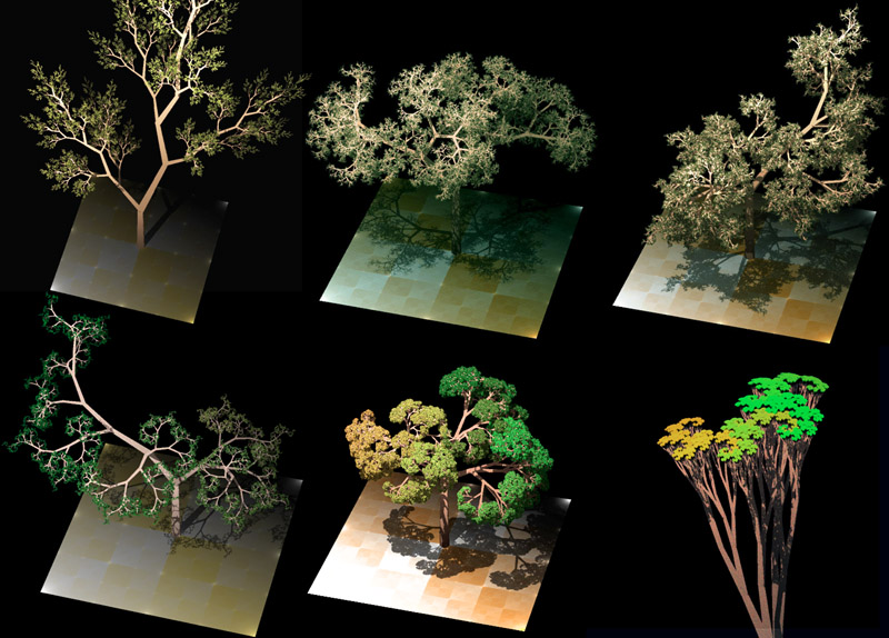
By changing parameters such as numbers, angles, and lengths of branches, we can make various look of trees. Similar to a real tree, we don’t want the tree to grow infinitely. We can halt the process at an arbitrary number of steps.

枝の数、角度、長さなどのパラメータを変更することで、異なる見た目の木を作成することができます。本物の木と同じき無限に成長されると困るので、適当なステップ数でプロセスを止めることにします。

Mathematically speaking, a fractal must have infinite details. But it doesn’t matter much as we are more interested in using the concept to sketch something interesting.
数学的に言うとフラクタルには無限の詳細が存在する必要があります。しかし、概念を使って何か面白いものをスケッチする目的からすると、厳密さはあまり重要ではありません。

If you’re interested, check out L-system (Lindenmayer system). An L-system is a string-based system often used to create tree-like structures with a set of rules such as ‘start from A’, ‘replace A with AB’, and ‘replace B with A’. You can think of it as a fractal defined through string processing. This algorithm is frequently implemented in 3D modeling programs.

興味があれば、L-system（Lindenmayer system）について調べてみましょう。L-systemは、「Aから始める」、「AをABに置き換える」、「BをAに置き換える」といったルールの集合によって木のような構造を作るためによく使われる文字列ベースのシステムです。文字列処理を通じて定義されたフラクタルとも言えるでしょう。このアルゴリズムは、3Dモデリングのプログラムによく実装されています。

https://en.wikipedia.org/wiki/L-system#/media/File:Dragon_trees.jpg

Hausdorff dimension ハウスドルフ次元

This section is a slight detour, as I’ve never used this concept in practical applications. Nevertheless, it’s a fascinating concept that redefines our understanding of dimensionality.

このセクションはちょとした寄り道です。これを実用で使ったことはありませんが、ハウスドルフ次元は次元に関する理解を再定義するという意味でとても面白い概念です。

The Hausdorff dimension is a measure that captures an aspect of fractal shapes, abstracting or expanding the concept of dimensions with which we are familiar (like 2D, 3D). Among the different meanings and characteristics “dimensions” have, it specifically focuses on how the size of a shape changes with scale.

ハウスドルフ次元は、フラクタルの持つ性質のある一面を図るための値で、お馴染み次元の概念（2D、3Dなど）を抽象化または拡張したものです。 「次元」が持つ様々な意味や特性の中でも、特に形状の大きさが拡大、縮小によってどう変化するかに焦点を当てています。

Imagine a square, cube, or any equivalent in a dimensional world. If you scale the length of sides by $n$, the size of the object, i.e., the area in 2D, the volume in 3D, becomes $n^{\text{the number of dimensions}}$. For example, if you double the sides of a cube, the volume will increase by $2^3=8.$ This rule holds for any other shapes. But that mathematically true fractals with infinite steps of self-replications don’t follow this rule.

正方形、立方体、または多次元世界におけるその仲間を想像してください。辺の長さのを$n$倍に拡大すると、物体の大きさ、つまり2Dにおける面積、3Dお体ける積は $n^{\text{次元数}}$ になります。例えば、立方体の各辺を2倍にすると、体積は $2^3=8$ に増加します。これは他のどんな形状にも当てはまりますが、無限の自己複製ステップを持つ数学的に厳密なフラクタルはこのルールに従いません。

Let’s calculate the case of the Sierpinski carpet for example. If we triple the scale of the Sierpinski carpet, the new carpet is composed of 8 copies of the original, meaning the area has increased by a factor of 8, instead of 9 ($3^2$ for 2 dimensions). This relationship can be written as below, where $D$ represents the Hausdorff dimension:

例として、シェルピンスキーカーペットの場合を計算してみましょう。シェルピンスキーカーペットを3倍に拡大すると、新しいカーペットは元のカーペットの8つのコピーで構成されるので、面積は9（2次元の場合の$3^2$）ではなく8倍になります。この関係は下のように書くことができ、ここで$D$がハウスドルフ次元になります。

$8=3^D$

${\begin{aligned} D = \frac{\log(8)}{\log(3)} \end{aligned}}$

Solving this equation gives us approximately 1.89. Roughly speaking, the Hausdorff dimension of the Sierpiński Carpet is slightly less than 2 because a fraction of the space is removed through the infinite repetition of the process. The Koch curve is the opposite. You can think of it as based on a 1D shape (though it is drawn on a plane, it is essentially a series of line segment) that gains some extra length with each of the infinite steps. The Hausdorff dimension of the Koch curve is about 1.26, a little higher than 1.

この方程式を解くと、およそ1.89になります。ざっくり言うと、シェルピンスキーのカーペットでは2Dの形状から無限回のプロセスを通じて空間の一部を取り除くので、ハウスドルフ次元が2よりもわずかに低いです。コッホ曲線はその逆です。コッホ曲線は 1次元をベースにした形だと考えられ（平面上に書かれていますが、実質は線分の集まりです）、無限のステップごとに少しずつ追加の長さを得ていきます。コッホ曲線のハウスドルフ次元は約1.26で、1よりもわずかに高くなります。

Fractal Noise フラクタルノイズ

The randomized Koch Curve resembles a coastline. Abstractly, the process can be seen as replacing parts of a curve with smaller curves. This method, or more practically, starting from a large-scale curve and recursively adding smaller-scale curves, is commonly used to emulate natural looks and behaviors.

ランダム化したコッホ曲線は、海岸線に似ていました。これを抽象化すると、曲線の一部をより小さな曲線で置き換えるプロセスとして捉えられます。この手法、より実践的には、大きな曲線から始めてより細かな曲線を再帰的に加える方法は、自然な見た目や振る舞いを模倣するためによく用いられます。

For features like coastlines or mountain ridges, we need some randomness. We also want the change to be continuous to appear natural at various scales. Noise functions are an ideal fit for a case like this. As discussed in Taming Randomness, noise, in the context of computer graphics and simulations, refers to random or semi-random data used to generate textures or patterns.

海岸線や山脈のような特徴には、ある程度のランダムさが必要です。また、様々なスケールで自然に見えるよう、変化は連続的である方が良いでしょう。こうしたケースにはノイズ関数が最適です。ランダムさを手なづけるのページで触れたように、コンピュータグラフィックスやシミュレーションの文脈では、ノイズとはテクスチャやパターンを生成するために使用されるランダムまたは、ランダムらしいデータを指します。

In the examples of the Sierpiński carpet or Koch curve, we used discrete units for the process and replaced each part of the unit with a smaller copy of itself. Because a noise function is continuous, and we want the result to be continuous too, we can add up different scale of noise instead of splitting a line into pieces and replacing them. The draw (very loosely) illustrates how this is an extension of the process for the Koch curve.

シェルピンスキーカーペットやコッホ曲線のプロセスでは、バラバラ（離散的）なユニット（単位となる形状）を用いて、そのユニットの各部分をそれ自体の小さなコピーに置き換えました。 ノイズ関数は連続的で、結果も連続である方が良いので、ラインを分割して置き換えるのではなく、異なるスケールのノイズを加算することにします。 下のイラストはこの方法がなぜコッホ曲線の手法の拡張と言えるのかを（とてもざっくり）描いたものです。

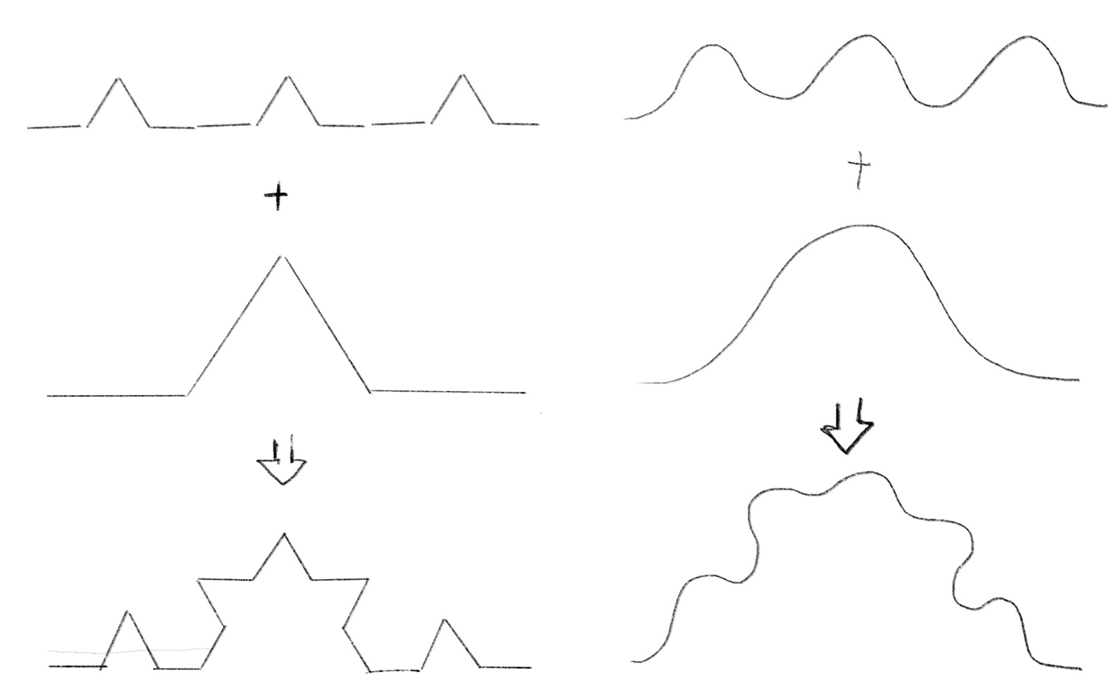
Take a look at the demo below. The curve at the top is the sum of the three other curves below it. We start with a large wavy shape, then create a scaled-down version (or increased frequency) of the same shape and add it to the original wave, then repeat.

下のデモをご覧ください。一番上に上の曲線は、その下にある3つの曲線を足し合わせたものです。大きな波形から始めて、同じ形状を縮小したもの（または周波数を増やしたもの）を作り、それを元の波に加え、それを繰り返します。

These repetitions are called octaves, analogous to musical octaves where the frequency doubles per octave. At the top of the code, three variables define the number of octaves and how the amplitude and frequency change per octave.

音楽ではオクターブごとに周波数が倍になることに対する類似から、これらの繰り返しはオクターブと呼ばれます。コードの冒頭には、オクターブの数、およびオクターブごとの振幅と周波数の変化を定義する3つの変数があります。

const nOctaves = 3; // The number of noise octaves
const freqMult = 4; // Multiplier for the frequency per octave
const ampScale = 0.25; // Multiplier for the amplitude per octave

Each octave adds a layer of noise that is smaller in amplitude and higher in frequency than the last. This creates a more complex and detailed pattern. Try adjusting these values to see how they influence the results. This example uses the noise() function from p5.js, but you can combine any function at any scale.

それぞれのオクターブが、ひとつ前のオクターブよりも小さな振幅と高い周波数のノイズのレイヤーを加えていくことで、より複雑で詳細なパターンが作成されます。これらの値を調整して、結果にどんな影響を与えるか見てみましょう。この例ではp5.jsのnoise()関数を使っていますが、どんな関数でも好きなスケールで組み合わせることができます。

The demo below creates 2D fractal noise with a GLSL shader. The left side shows the value directly as the brightness. The right side interprets the value as the height, and applies simple diffuse lighting to render a terrain. For the implementation the noise function in GLSL, refer to the Book of Shaders’ Noise page.

下のデモはGLSLシェーダーを用いて2Dのフラクタルノイズを生成します。左側には値を明るさとして直に表示し、右側では値を高さと解釈して、シンプルなディフューズライティングを用いて地形をレンダリングします。 GLSLでのノイズ関数の実装については、Book of Shadesのノイズのページを参照してください。

Implementing the Mandelbrot set マンデルブロ集合の実装

To conclude this page, let’s examine the mathematics behind the Mandelbrot set. We saved this for the end because the concept of self-similarity is far more important, and the specific mathematics for the Mandelbrot set could be distracting. But having looked through all the examples, we are ready to appreciate how a simple set of formulas can create a very complex shape with infinite details.

このページの締めくくりとして、マンデルブロ集合の背後にある数学を見てみましょう。これを最後まで取っておいたのは、自己相似性の概念の理解する方がずっと重要で、そのためにはマンデルブロ集合の具体的な式は邪魔になるからです。しかし、すべての例を見てきた今、シンプルな数式が無限のディティールを持つ非常に複雑な形状を作り出す様子を楽しむ準備ができたと言えるでしょう。

The Mandelbrot set is defined as a set of complex numbers that satisfy a certain condition. But from a graphical perspective, you can think of it as a process of taking points on a 2D plane and deciding whether each point should be drawn on the canvas.

マンデルブロ集合は、特定の条件を満たす複素数の集合として定義されます。グラフィカルな視点から見ると、2Dの平面から任意の点を選んだ時に、その点をキャンバスに描くかどうかを決めるプロセスとも考えることができます。

Below is the formula for the Mandelbrot set.

下がマンデルブロ集合の公式です。

$z_0 = 0$

${\begin{aligned} z_{n+1} = z_n^2 + c \end{aligned}}$

The complex number $c$ can be written as $x + iy$ ($i$ is the imaginary unit - See this page for more about complex numbers.) If you consider $x$ and $y$ as coordinates, you can view the complex number as a point on a plane. Take a point on the plane and apply it to the formula above. If it diverges to infinity, the complex number, or the point, doesn’t belong to the Mandelbrot set. If it converges to a certain number, it belongs to the set. Let’s take a point $(3, 2)$, ie., $c=3+2i$ as an example.

複素数$c$は$x + iy$と書くことができます（$i$は虚数単位です。複素数についてはこちらのページもどうぞ）。$x$と$y$を座標と考えると、複素数を平面上の点として見ることができます。平面上から点を選んで上の式に適用してみましょう。結果が無限大に発散する場合、その複素数、つまりその点はマンデルブロ集合に属していません。結果が収束する場合、その点は集合に属しています。例として、点$(3, 2)$、つまり、$c=3+2i$ について調べてみましょう。

$z_0 = 0 \ z_1 = z_0^2 + c = 0^2 + 3 + 2i = 3 + 2i \ z_2 = z_1^2 + c = (3 + 2i)^2 + 3 + 2i = 8 + 14i \ z_3 = z_2^2 + c = (8 + 14i)^2 + 3 + 2i = -129 + 114i \ z_4 = z_3^2 + c = (-129 + 114i)^2 + 3 + 2i = 3684 - 29410i$

You can see this grows very quickly. It does diverge to infinity, so the point $(3, 2)$ doesn’t belong to the set.

計算結果がとても速く増えている様子がわかります。この結果は実際に無限大に発散するので、点$(3, 2)$は集合には属しません。

The demo below essentially runs this process for every pixel on the canvas. Because we cannot repeat the steps infinitely in practice, we use an arbitrary threshold if(length(z) > 2.0) break;as an approximation. The code iterates the steps a maximum of 100 times to measure how quickly it diverges. If it doesn’t go over the threshold after 100 iterations, it is not likely to diverge, and the pixel becomes white. If the value exceeds the threshold, the pixel gets darkened according to how quickly it does so.

下のデモは実質、キャンバス上のすべてのピクセルでこのプロセスを実行します。現実には無限にステップを繰り返すことはできないので、近似値として適当な閾値 if(length(z) > 2.0) break; を使います。このコードは、収束の速さを測定するために、最大100回までステップを繰り返します。100回の繰り返し後も閾値を超えない場合は発散しない可能性のでピクセルを白く塗ります。閾値を超える場合にはその速さに応じて、ピクセルを暗くしていきます。

If you see a formula that is hard to grasp intuitively, it is a great idea to visualize it with code. Rather than applying a threshold, the demo below renders the value of $c$ by mapping $x$ and $y$ to the red and green channels. Can you see that it gains more fidelity and detail around the edge as the number of iterations increases? What other observations can you make from this visualization? Can you think of other ways to further investigate the Mandelbrot set?

式が直感的に理解しにくい場合にはコードで視覚化してみましょう。下のデモでは閾値を適用する代わりに$c$の値を、$x$と$y$をRとG チャンネルにマッピングすることで直接レンダリングします。反復回数が増えるにつれて、形のエッジがクッキリと詳細になっていく様子が見えるでしょうか。他には何が読み取れるでしょう。マンデルブロ集合を調べる他の方法を考えてみましょう。