Integration 積分

Take a look at the demo of the falling apple from the differentiation page again. The rate of change of the position is velocity, and the rate of change of velocity is acceleration. We can think about this the other way around. The position of an object at a certain moment is a result of the effect of velocity accumulated over time, and the velocity at a certain moment is a result of the effect of acceleration accumulated over time.

微分のページから、落下するリンゴのデモをもう一度見てみましょう。位置の変化の割合は速度で、速度の変化の割合は加速度でした。これを逆向きに考えることもできます。つまり、ある瞬間の物体の位置は一定時間の間の速度の影響が積み重なった結果で、ある瞬間の速度は一定時間の間の加速度の影響が積み重なった結果だと考えることができます。

For example, if a car has been moving at 100 km/h toward east for 2 hours, it must be at 200 km east from its starting point. This is the basic idea of integration. An integral represents the accumulation of the rate of change over a certain span. Differentiation relates to ‘difference’, capturing the rate of change at each moment, while Integration ties to ‘sum’, accumulating these changes over time. In fact, the origin of the symbol of integral $\int$ is the elongated “S,” which stands for “summa” in Latin, meaning “sum” or “total.”

例えば、車が東へ時速100キロの「速度」で2時間進み続けた場合、出発点から200キロ東の「位置」に来るはずです。これが積分の基本的な考え方です。積分は、ある期間の間の変化率が積み重なったものを表します。微分は「差」に関係しており、瞬間の変化率を捉えます。一方、積分は「和」に関係しており、変化を時間の経過に対して累積します。実際に、積分の記号 $\int$ は、長く引き伸ばしたSの形をしており、ラテン語の「summa」、「総和」という意味の言葉から来ています。

Integration doesn’t always have to be about position and time, but we’ll stick with this example for now as it is the most intuitive.
積分は必ずしも時間や位置に対する問題でなくて良いのですが、今はこの例を最も直感的な例として用いることにします。

Area and Integration

面積と積分

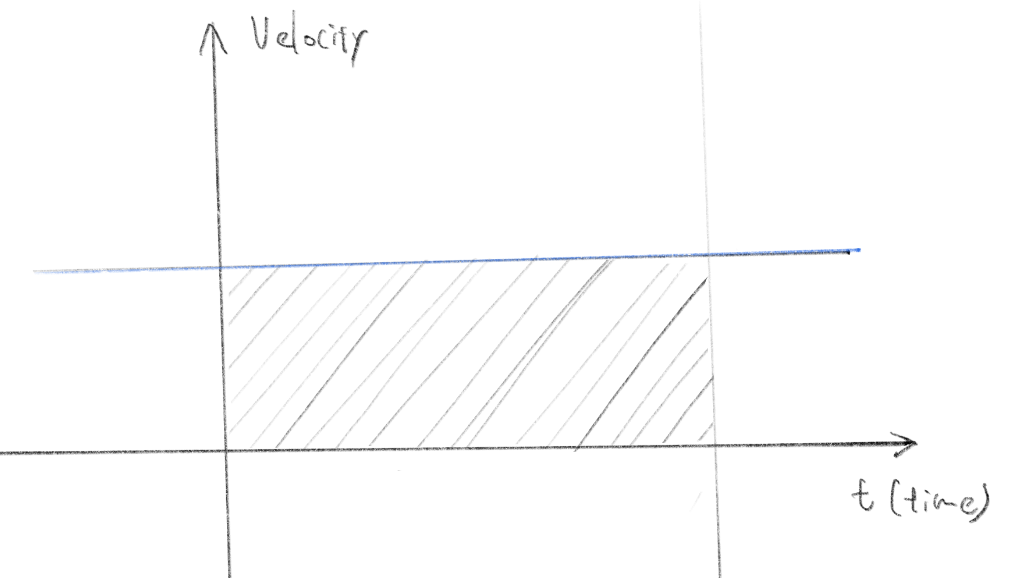
Integration can also be thought of as the area under the graph. Let’s consider the relationship between velocity and position as an example. If the velocity is constant, the change in position is simply the product of velocity and time. It is clear that it corresponds to the area of the shaded part of the graph below.

積分はグラフの面積として考えることもできます。速度と位置の関係を例に考えてみましょう。速度が一定であれば、位置の変化は速度に時間を掛け合わせるだけなので下のグラフの斜線部分の面積に相当することは明らかです。

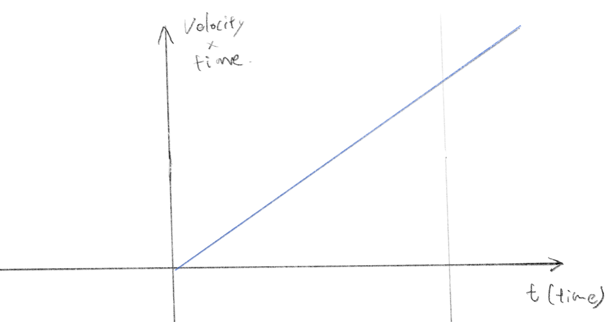
If we plot the graph of the area, it will look like this. This is the graph of the integral of velocity, which represents the change in position over time. When the velocity is constant, the position graph becomes a straight line.

面積のグラフを描くと、このようになります。これは速度の積分のグラフであり、時間に対する位置の変化を表しています。もし速度が一定であれば、位置のグラフは直線になります。

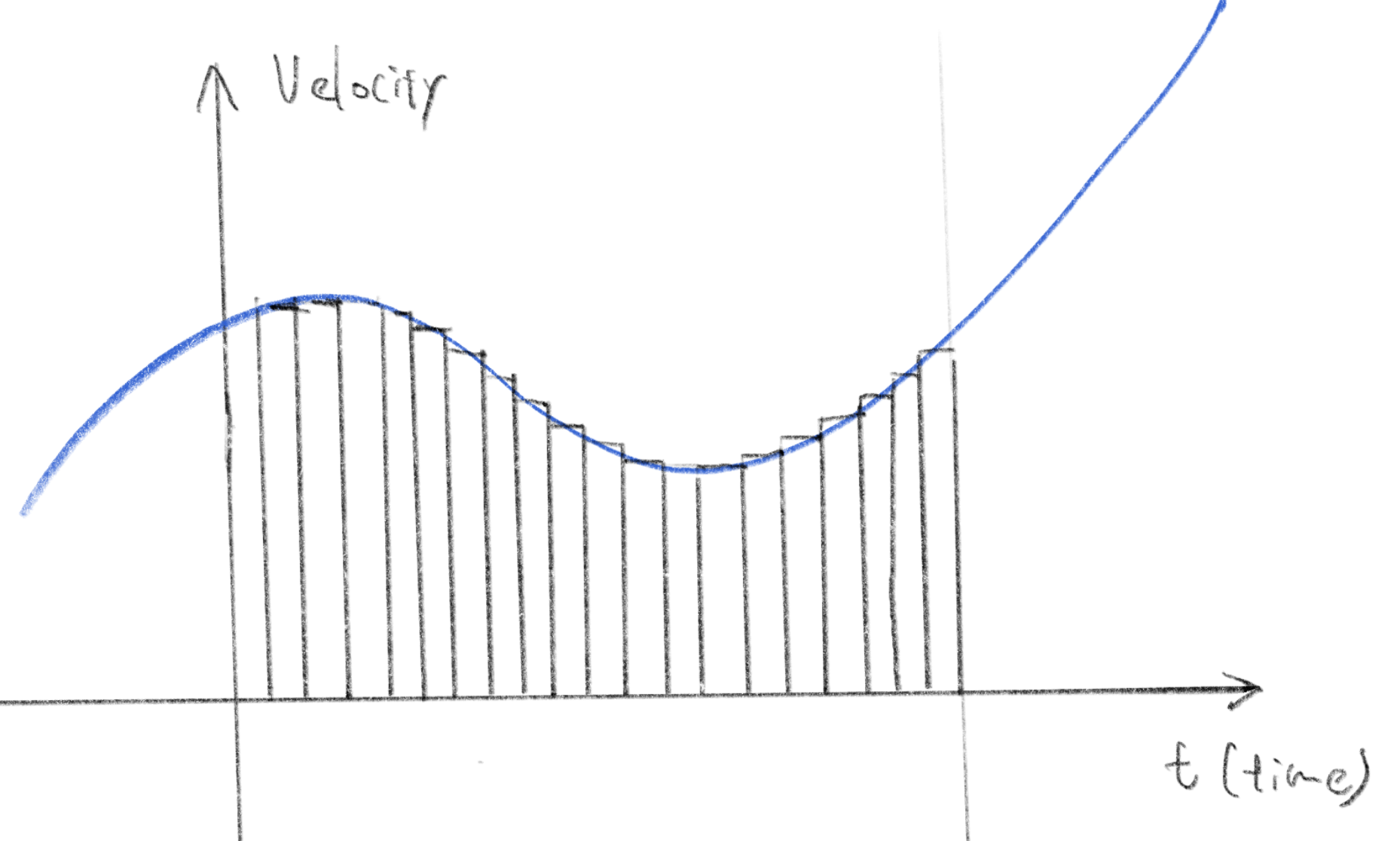
It may not be that obvious when the graph is not straight. But if you imagine that the shape consists of many narrow rectangle strips, you can approximate its area. Integration is the accumulation of change over time. You can think of each strip as an approximation of the effect of velocity over a short amount of time. By summing up the areas of all the strips, you can find the total amount of change.

曲線の場合そこまで単純にはいきませんが、グラフの形がたくさんの細長い長方形の帯で構成されていると考えれば、面積を近似できます。積分とは、時間の経過に伴う変化の蓄積なので、それぞれの帯が短かい時間の間の変化を近似したものだと考えられます。全ての帯の面積を合計すれば、変化量の全体を求めることができます。

Numerical Integration

数値積分

In ordinary math books, the next step would be to make these strips infinitely narrow, bringing them infinitely closer to the original graph shape. But, when using integration on a computer, it is often more practical to approximate it by choosing a sufficiently small width for the strip.

普通の数学の本なら、次のステップでこの帯を無限に狭くして帯の集まりがグラフの形に限りなく近づくようにします。ですがコンピュータで積分を使う場合、十分に狭い帯の幅を選んで近似する方が実用的な場合がよくあります。

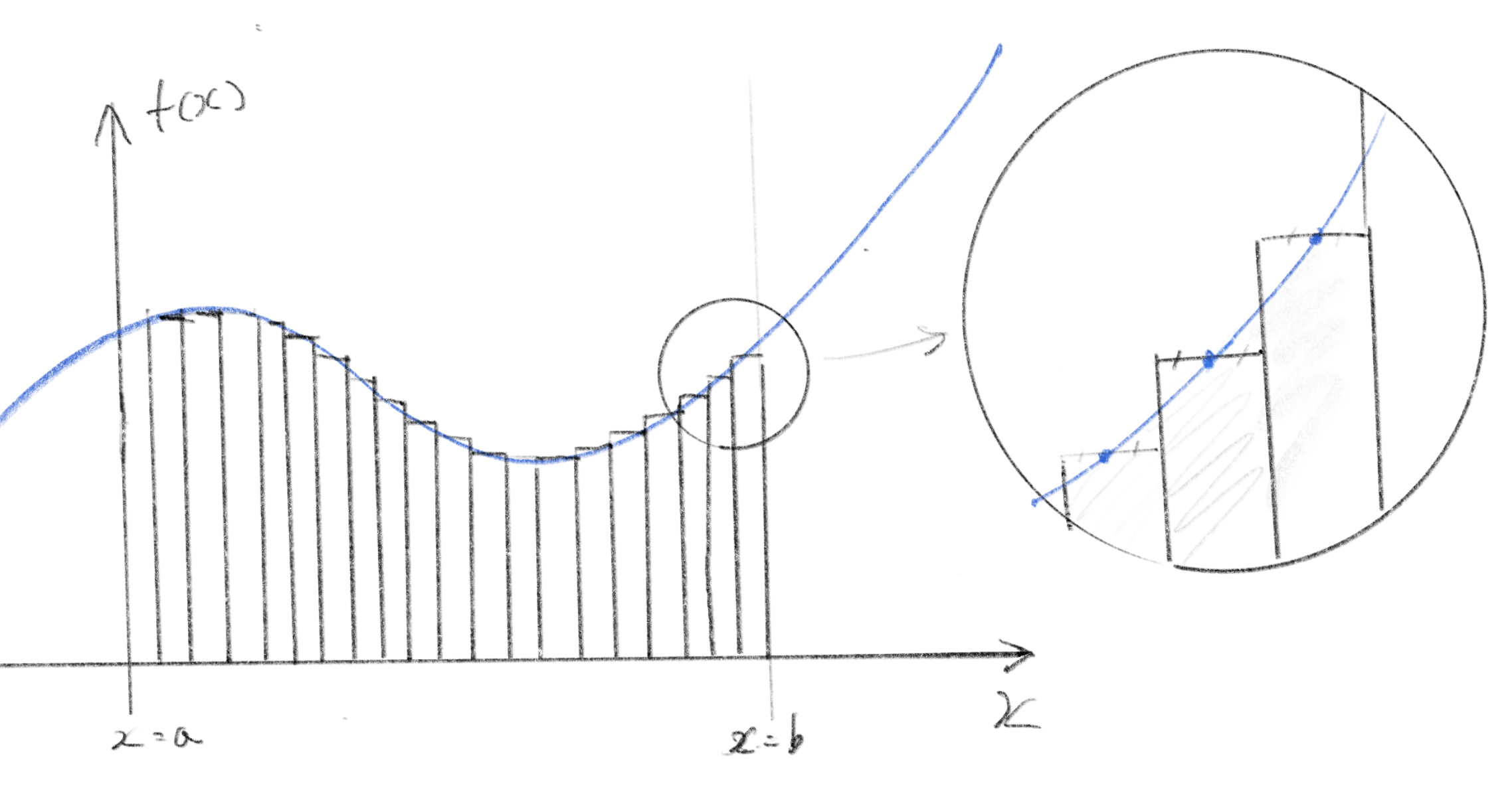
We are going to approximate the integral of a function $f(x)$ . To calculate the sum of the areas of strips, we need to decide where to start and end. For example, if you want to know how far a car travels from a function that represents its velocity, you need to determine the starting and ending times for the measurement to be complete.

ある関数 $f(x)$ の積分を近似してみましょう。帯の面積の合計を計算するには、始まりと終わりを決める必要があります。例えば、車の速度を表す関数から車がどれだけ移動するかを知りたい場合には、始める時刻と終える時刻を決めないと測定が終わりません。

Let’s say we start from $x=a$ and end at $x=b$ . We need to decide the width of each strip or how many strips we want to divide the range between $a$ and $b$ into. Let’s call the number of strips $n$ . Then, the width of each strip $\Delta x$ is $\displaystyle {\begin{aligned} \frac{b-a}{n} \end{aligned}}$ . We will use the value of $f(x)$ at the center of each strip as the height. We can write this as:

ここでは $x=a$ から始めて $x=b$ で終わるものとします。帯の幅か、 $a$ と $b$ の間を幾つに分割するかも決める必要があります。 $a$ と $b$ の間の帯の数を $n$ とすると、帯の幅 $\Delta x$ は $\displaystyle {\begin{aligned} \frac{b-a}{n} \end{aligned}}$ となります。それぞれの帯の高さは、その中心の $f(x)$ の値を使います。これは下のように書くことができます。

$\Delta$ is a symbol used to represent a small yet finite change.
$\Delta$ は有限の小さな変化を表す記号です。

$x$ at the center of the strip

帯の中心の $x$ の値

${\begin{aligned} a + (i+\frac 1 2) \Delta x \end{aligned}}$

The area of a single strip

帯のひとつ分の面積

${\begin{aligned} f(a + (i+\frac 1 2)\Delta x)\Delta x \end{aligned}}$

The total area of all strips

全ての帯の面積の合計

${\begin{aligned} \sum_{i=1}^{n} f(a + (i+ \frac 1 2)\Delta x)\Delta x \end{aligned}}$

Take a look at the Summation page if you are not familiar with $\sum$ (sigma).
$\sum$ (シグマ)に馴染みがない場合は総和のページを見てください。

In JavaScript:

JavaScriptで書くとこうなります。

function integral(f, a, b, n) {
    let delta = (b - a) / n;
    let sum = 0;

    for (let i = 1; i <= n; i++) {
        let xi = a + (i + 0.5) * delta;  // midpoint of the i-th subinterval
        sum += f(xi);
    }

    return sum * delta;
}

// Example usage:
const f = x => x * x;  // Define your function here
const result = integral(f, 0, 1, 1000);  // Approximates the integral of x^2 from 0 to 1 with 1000 subintervals
console.log(result); //0.33433425 - close to the correct answer 0.3333...

The following demo shows the graph of a function that uses p5js’s noise and its integral. The graph on the left shows the noise function, while the graph on the right represents the integral of that function. In other words, the graph on the right shows the accumulated value, or the area of the graph on the left, from point 0 up to point x on the x-axis. Clicking on the canvas will randomly update the function. Note that when the function value goes negative, the graph of the integral will also change in the downward direction. It is important to be aware that there can be negative areas in the integral. Since the integral function is expensive due to the for loop, it is modified to calculate the values beforehand and return a function.

下のデモではp5jsのnoise関数を使った関数とその積分のグラフを並べて表示しています。左がノイズ関数、右がその積分です。言い換えると、右側のグラフは、左側のグラフのx軸上で点0から点xまでの範囲の値を積み重ねたもの、または面積を表しています。キャンバスをクリックすると関数がランダムに変わります。関数の値がマイナスになる場合は積分のグラフも下に向かって変化することに注意してください。積分ではマイナスの面積が存在するわけです。integral関数はforループによる計算量が多いので、先に値をまとめて計算して関数を返すように変更しました。

This method of approximating integrals using a numerical technique is called “numerical integration”. The particular technique we used above is known as the midpoint rule or rectangle method. If you’re interested, there are various other techniques for numerical integration that you can look up. You can also compare this method to numerical differentiation, which we discussed on the differentiation page.

この数値的な手法による積分の近似は、「数値積分」と呼ばれています。上で使った具体的な手法は中点則または長方形法と呼ばれます。数値積分には様々な手法があるので興味があれば調べてみましょう。また、微分のページで見た数値微分の手法と比べることもできます。

Euler Method

オイラー法

In computer games or animations, we often use a simple Euler method to update the position of an object frame by frame. This involves adding the velocity (or velocity multiplied by time) to the current position every frame. This method, which you might already be familiar with, can also be seen as a numerical approximation of an integral.

コンピューターゲームやアニメーションではよく、簡単なオイラー法を使ってオブジェクトの位置をフレームごとに更新します。この手法ではフレームごとに、速度（または時間に速度を掛けたもの）を現在の位置に加算します。このおなじみの手法も数値積分の数値的な近似と考えることができます。

There are improved versions of the Euler method, such as the Runge-Kutta method, which can be also considered as numerical integration techniques. To learn more about these methods, read the following pages and compare them with the method we discussed here.

オイラー法の改良版としてルンゲ＝クッタ法などがありますが、これらも数値積分として考えることができます。これらについては以下のページを読んで、このページの手法と比較してみましょう。

Newtonian mechanics ニュートン力学

Continuous Time and Discrete Time 連続した時間とバラバラな時間

Notation of Integration

積分の表記法

We could have ended this page already since we have covered most of what we need to practically implement integration. However, in order to read documents written in proper mathematical language, it would be useful to learn a few more things. First, let’s see the notation of integration.

積分の実用的な実装に必要な内容はほとんどカバーしたのでこのページを終わりにしても良いのですが、きちんとした数学の表現で書かれたドキュメントを読むために知っておいた方が良いことがいくつかあります。まずは積分の表記法を見てみましょう。

The below is the simplified version of the numerical integration we have been discussing. In the expression, $n$ is the number of the strip, $\Delta x$ is the width of the strip (indicating a small change along the x-axis), and $f(x) \Delta x$ is the area of each strip. This represents the idea of dividing the graph into $n$ strips and add them up.

下の式は、これまで見てきた数値積分をシンプルにしたものです。式中の $n$ は帯の数、 $\Delta x$ は帯の幅（x軸上の小さな変化）、 $f(x) \Delta x$ はそれぞれの帯の面積です。これはグラフを $n$ 個の帯に分けて合計するという考え方を表しています。

$\begin{aligned} \sum_{i=1}^{n} f(x) \Delta x \end{aligned}$

The integral of a function $f(x)$ between $x = a$ and $x = b$ is typically denoted as below.

関数 $f(x)$ の $x = a$ から $x = b$ までの積分は普通下のように書きます。

$\begin{aligned} \int_{a}^{b} f(x) , dx \end{aligned}$

The integral (not approximated) is the continuous accumulation of the values of the function $f(x)$ over the interval $[a, b]$ multiplied by an infinitely small width $dx$ . It represents a very similar idea to the summation version above, but in this case, we are thinking about it as a continuous change or an infinite number of strips. In the notation of integration, we only specify the beginning and end ( $a$ and $b$ ) without mentioning the number of strips.

（近似ではない本来の）積分は、関数 $f(x)$ の値を区間 $[a, b]$ 上で連続的に累積して、無限に小さな幅 $dx$ を掛けたものです。これは上の総和を使ったバージョンにとても良く似た考え方ですが、この場合は連続的な変化または無数の帯として考えています。積分の表記法では、帯の数には触れず始点と終点（ $a$ と $b$ ）のみを指定します。

We can see the similarity in the symbols themselves. As already mentioned, $\int$ is an elongated “s” and comes from “summa” with is a latin word for “sum”. $\Sigma$ is the capital of a Greek letter sigma and represents summation.

記号自体もよく似ています。既に触れたように $\int$ は上でも引き延ばした「s」の形で、「summa」というラテン語で合計（sum）を表す言葉に由来しています。 $\Sigma$ はギリシャ文字のシグマの大文字で、総和を表します。

Definite integral and Indefinite integral

定積分と不定積分

The integral we have been discussing, which provides the accumulated change or the area between the curve and the x-axis within a certain interval, is known as a “definite integral”. The definite integral gives you a numerical value as the result. There is another closely related concept called the “indefinite integral”, which gives you a function instead of a specific number.

ここまで見てきた、特定の範囲の間で曲線とx軸の間の変化の蓄積や面積を求める積分は「定積分」と呼ばれます。定積分の結果は数値になります。関連する概念に、「不定積分」という特定の数値ではなく関数を返すものがあります。

On the differentiation page, we learned that differentiating a function yields a new function. For instance, the derivative of the function $f(x) = x^2$ is $f’(x) = 2x$ . This means that the slope, or rate of change, of $f(x) = x^2$ for any point $x$ is $2x$ . The inverse of this process - finding a function that represents the total change or area the graph from the function of the rate of change describes (like deriving a position function from a velocity function) - is the indefinite integral. Using the same example, the indefinite integral of the function $f(x) = 2x$ is $\int f(x) dx = x^2 + C$ .

微分のページでは、関数を微分すると新たな関数が得られることを学びました。例えば、関数 $f(x) = x^2$ の微分は $f’(x) = 2x$ です。これは、 $f(x) = x^2$ のどの点 $x$ においても、その傾き、または変化率が $2x$ になるという意味です。この逆のプロセス、つまり（速度の関数から位置の関数を導くように）変化率を表す関数から、変化の総量、またはグラフの面積を表す関数を見つけることを不定積分と呼びます。同じ例を使うと、関数 $f(x) = 2x$ の不定積分は $\int f(x) dx = x^2 + C$ となります。

Did you notice that there is an additional constant $C$ . This constant signifies that several functions can have identical rates of change, with their differences being solely a constant value. When considering position and velocity, you can think of $C$ as the starting point of your function.

定数 $C$ が増えていることに気づいたでしょうか。これは、この定数値が異なるだけで変化率が同じ関数を複数ありえることを示しています。位置と速度を考える際には、 $C$ は関数の始点と考えることもできます。

To paint a concrete picture, think of a trip on a personal jet. While your jet’s velocity profile can be exactly the same, you could start from anywhere, such as Tokyo, Los Angeles, or Buenos Aires. Despite the velocity function and the resulting change in position being the same, your final destinations will be very different based on your origin. This difference in starting points is the $C$ .

より具体的にイメージするために、個人用ジェット機での旅行を考えてみましょう。ジェット機が同じ速度の変化を辿るとしても、出発地は東京、ロサンゼルス、ブエノスアイレスなど、様々な場所がありえます。速度の関数とそれによる位置の変化が同じでも、出発地によって最終的に全く違った場所に到着することになるでしょう。この出発点の違いが $C$ というわけです。

As the derivative of $x^n$ is $nx^{(n-1)}$ , the inverse, the indefinite integral of $x^n$ is $\begin{aligned} \frac 1 {n + 1}x^{n+1} \end{aligned} + C$ . There are many other known patterns. Try searching for “Integral formulas” or similar keywords.

$x^n$ の微分が $nx^{(n-1)}$ なのでその逆、 $x^n$ の不定積分は $\begin{aligned} \frac 1 {n + 1}x^{n+1} \end{aligned} + C$ になります。他にも多くのよく知られたパターンがあります。「積分の公式」といったキーワードで検索してみましょう。

Diffusion 拡散