Differentiation 微分
Differentiation is a useful tool for determining how fast something is changing, which is represented by the rate of change of a function or the slope of a graph. It’s key when you’re looking at movements, shapes, or physics simulations. That rate of change, or a function that stands for it, is what we call a “derivative”. The process of finding the derivative is called “differentiation”.
微分は、関数の変化の割合や、またはグラフの傾きによって表される、何かが変化する速さを調べるための便利なツールで、動き、形状、または物理シミュレーションを扱う場合には欠かせないものです。この変化の割合、または変化の割合を表す関数は「微分」と呼ばれ、導関数を見つけることは「微分する」と言います。
英語だとそれぞれを ”derivative”、”differentation”と別の単語で表すので気をつけてください。また日本語ではある関数を微分した結果得られる関数を「導関数」と呼ぶこともありますが、英語には直接対応する単語は無いようです。
This page has become a bit lengthy, but the main goal here is to show that the basic idea of differentiation is actually quite simple. At first glance, formulas involving derivatives can seem cryptic. However, especially when taking a numerical approach that we’ll look at, it’s just a matter of finding the difference between neighboring points and dividing that difference by the distance.
このページは少し長くなってしまいましたが、主な目的は微分の基本的な考え方が実はとてもシンプルだと示すことです。一見、微分を含む数式は難解に見えるかもしれませんが、特にこのページで取り上げる数値的なアプローチを取る場合、単に隣り合う点同士の差を求めて、距離で割るだけのことです。
I’m not saying that it’s trivial or that I fully understand the subject. In fact, it’s quite the opposite. I have only scratched the surface. But differentiation can be very powerful and useful just by understanding the basics and learning a few simple practical methods.
微分が取るに足らないものだったり、既に完全に理解したと言っているわけではありません。実際はその逆で、ほんの表面をかいつまんでいるだけなのですが、それでも基本を理解し、いくつかのシンプルな実用的な方法を学ぶだけで、微分は非常に強力で役立つものになります。
Rate of Change
変化の割合
Think of an apple falling straight downward. From the starting point, the apple’s position changes moment by moment, moving downward. The rate of change of the apple’s position with respect to time is its velocity. Velocity can be defined as the derivative of position with respect to time. As the apple falls, not only does its position change, but its velocity also increases due to gravity. The derivative of velocity with respect to time is called acceleration, which represents how much the velocity changes at any given moment. In this example, the gravity acting on the apple is constant, so the acceleration also remains constant.
リンゴが真っ直ぐ落下する様子を考えます。スタート地点から下に向かって、リンゴの位置は刻一刻と変化します。時間に対するリンゴの位置の変化の割合がリンゴの速度です。この時、速度は位置の時間に対する微分だと言うことができます。位置が変化するだけでなく、リンゴは重力に引かれて速度を上げていきます。速度の時間に対する微分は加速度と呼ばれ、その瞬間にどれくらい速度が変化しているかを表します。この例ではリンゴに働く重力の大きさは一定なので、加速度も常に一定になります。
| Change of position | → Differentiate → | The rate of change of position = Velocity = The slope of the graph of position |
| Change of velocity | → Differentiate → | The rate of change of velocity = Acceleration = The slope of the graph of velocity |
| 位置の変化 | → 微分 → | 位置の変化の割合=速度=位置のグラフの傾き |
| 速度の変化 | → 微分 → | 速度の変化の割合=加速度=速度のグラフの傾き |
The rate of change can be measured not only over time, but also over space. For example, the slope of a hill indicates the rate at which height is changing relative to the horizontal position. Therefore, it is the derivative of height. If we know the derivative of temperature relative to position, we may be able to predict the flow of wind.
変化の割合は時間に対してだけでなく、空間に対してでも構いません。例えば斜面の傾きは水平方向の位置に対して高さがどれくらいの割合で変化しているかを示しているので、高さの微分です。気温の微分、つまり位置に対する気温の変化がわかれば風の流れを予測できるかもしれません。
The term “gradient” is used when considering changes in values in a multi-dimensional space, such as the distribution of room temperature. It is not difficult, as we can consider each axis as a one-dimensional differentiation, but it is useful to remember the word and symbol. We will briefly touch on this at the end of this page.
部屋の気温の分布のように多次元空間での値の変化を考える場合は勾配(Gradiation)という言葉を使います。軸ごとに分けて一次元の微分として考えられるので特に難しいことはありませんが、言葉と記号は覚えておいた方が良いでしょう。このページの最後で簡単に触れます。
As you can see, the word “differentiation” is closely related to “difference.” The basic idea is that if something changes, you can calculate the amount of change by subtracting the value before from the value after. The only thing to keep in mind is that you need to consider the time it took for the change in order to determine the rate of change. To find the rate of change at a specific moment or point, especially, you need to consider the change over an infinitely small span. We will see this more precisely in the next section.
微分を表す英語 “differentiation” は、差 “difference” に深く関連しています。大元の発想は、何かが変化した時に、変化量は変化前の値と変化後の値との差になるということです。ただし、変化の割合を求めるには、変化にかかった時間を考慮する必要があります。特に、ある瞬間や点で変化率を求めるには、とても(無限に)小さな範囲での変化を考える必要があります。この点については、次の節でより正確に説明します。
Basics of Differentiation
微分の基礎
Let’s start from a very simple example. In the demo below, a small circle moves to the right at a constant velocity.
非常に簡単な例から始めましょう。下のデモでは、小さな円が一定速度で右に移動します。
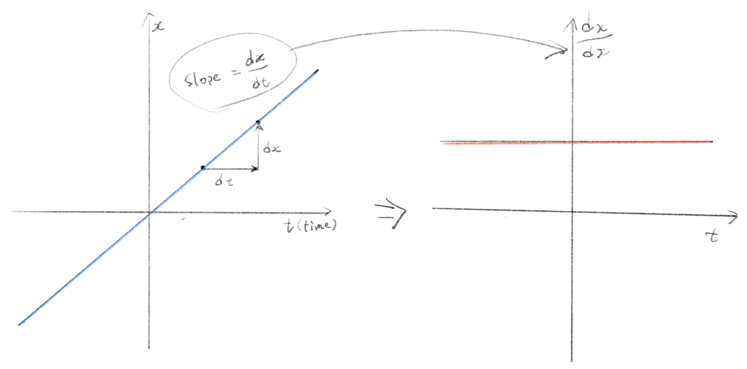
If we plot this with x-coordinate on the vertical axis and time on the horizontal axis, it becomes a straight line sloping upwards. To draw the graph of the derivative, which is the velocity, we need to determine the slope of this graph. The slope is the ratio of the change in the vertical axis to the change in the horizontal axis. For example, if increases by 500px in 5 seconds, the slope is 500 / 5, which is 100px/s. In this example, since it is a uniform motion, the slope is the same regardless of where it is taken, and the graph of the velocity is a horizontal straight line. The derivative of the velocity is the acceleration, but in this case, since the velocity does not change, the slope is zero everywhere, resulting in a zero slope.
これを座標を縦軸に、時間を横軸に取ってグラフに描くと右上がりの直線になります。この微分、つまり速度のグラフを書くにはこのグラフの傾きを求める必要があります。傾きは縦軸の変化量を横軸の変化量で割ったものになります。例えば5秒の間にが500px増えていれば、傾きは 500 / 5 で 100px/s です。この例は等速度運動なのでどこをとっても傾きは同じ、速度のグラフは水平な直線になります。速度の微分は加速度ですが、この場合は速度が変化しないので、傾きはゼロになります。
It is easy when we are dealing with something that changes at a constant rate. But what about cases where the rate changes too?
一定の割合で変化するものを扱うのは簡単ですが、その割合自体が変化する場合はどうでしょう。
The demo below shows how the slope of changes with respect to . The slope of this graph represents the derivative. Let’s assume that the horizontal axis () represents time and the vertical axis () represents the position. On the left side of the graph, the slope descends towards the right, indicating a negative value. Therefore, the value of representing the position keeps decreasing until the slope becomes 0 at . On the right side, the slope gradually becomes steeper, and the increase in accelerates.
下のデモでは の傾きが に対してどう変化するかを示しています。このグラフの傾きが微分です。横軸(x)を時間、縦軸(y)を位置だと思って見てみましょう。この場合グラフの傾きは速度を表します。グラフの左側では傾きが右下がり、つまりマイナスなので、位置を表す y が減り続け x = 0 の時点で傾きが0、右側では傾きが次第に急になりyの増え方が加速していきます。
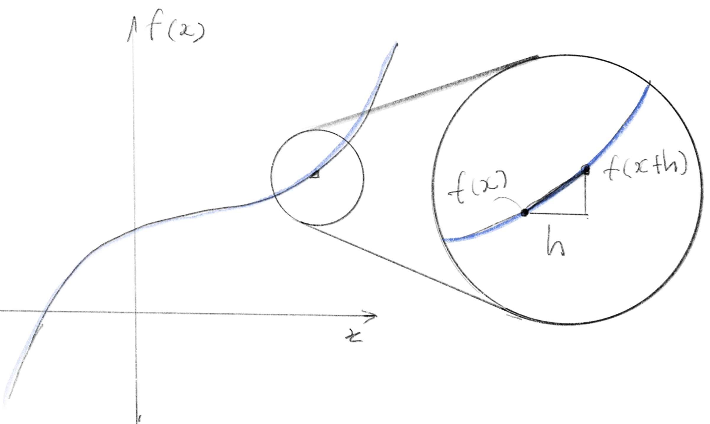
How can we find the slope of each point on a graph? The basic idea of differentiation is that a curve is very similar to a straight line when zoomed in. In the demo below, we zoom in on a point () on the graph of . We take two points on the curve and draw a straight line between them. While the points are far apart, the line and the curve look completely different, but if we shorten the distance between the points and look at a very narrow range, they are almost indistinguishable.。
グラフのある一点の傾きはどのように求められるのでしょうか。微分の基本的な考え方は、曲線は拡大すれば直線によく似ている、というものです。下のデモではのグラフのある一点() にズームしています。曲線の上で2点を取ってその間に直線を引きます。点が離れている間は直線と曲線は全く別物に見えますが、点と点との距離を縮めて非常に狭い範囲だけを見れば2つはほぼ見分けがつきません。
If we represent the idea of reducing the distance between two points indefinitely, mathematically, the derivative of a function is written as follows. means that approaches zero infinitely. The slope of the function at that point is the derivative, which is obtained by dividing the change of when is incremented by a small value from a certain point, by the change in (which is ).
この2点の距離を限りなく縮める考え方を数学的にきちんと表現すると、ある関数の微分は下記のように表されます。 は が限りなく0に近づくという意味です。ある地点からxをほん僅かにだけ増やしたときのf(x)の変化を、xの変化(つまり)で割ったものがその場所の関数の傾き、つまり微分になります。
There are several well-known patterns for differentiating functions, such as the general differentiation of which becomes . Applying this to gives the new function . The slope of at is , and at , it is . You can search, for example, for “differentiation formulas” to find many more examples.
関数の微分にはよく知られたパターンがいくつかあって、例えば一般に の微分は になります。これをに当てはめると という新しい関数が得られます。 の での傾きは 、 では といった具合です。「微分の公式」などで検索するとたくさん出てくるので調べてみましょう。
The demo below is a graph of the change of the slope, in other words, a graph of the derivative.
下のデモはこの傾きの変化をグラフにしたもの、つまり微分のグラフです。
Numerical Differentiation
数値微分
On this page, we won’t go into detail about how to find derivatives by manipulating equations. Instead, let’s try approximating derivatives using a computer. When dealing with complex and unpredictable phenomena, such as in physics simulations, it is not often straightforward to find derivatives by manipulating equations. Typically, it is more practical to use a method called numerical differentiation to find an approximate value.
このページでは式の変形で微分を求める方法については詳しくは触れません。その代わり、コンピュータを使って微分の近似をしてみましょう。物理シミュレーションなどで、複雑で予測しづらい現象を対象とする場合、式の変形で微分を求めることはあまりありません。大抵は数値微分という手法を使って近似値を求める方が実用的です。
Although not always highlighted in math textbooks, the technique of simply subtracting during differentiation is very widely used.
数学の教科書では必ずしも強調されていませんが、微分を単に引き算で計算する手法は広く使われています。
The essence of numerical differentiation is to replace the value of in the differentiation formula with a small number, rather than letting it approach zero. Let’s look at the original formula again.
数値微分の基本的な考え方は、微分の式のを無限に0に近づける代わりに、適当に小さな値で代用することです。元の式をもう一度見てみましょう。
For example, if and we set to 0.001, the numerical differentiation can be written as follows.
例えば の時 を0.001とすると、その数値微分は下のように書くことができます。
Let’s implement this in JavaScript.
JavaScriptで実装してみましょう。
const f = (x) => x * x;
const df = derivative(f);

console.log(df(1)); // 2.001 - Very close to the accurate derivative - 2

// Returns the derivative of the original function as a new function
function derivative(func) {
	  const h = 0.001; // The smaller the h, the more accurate the result becomes.
    return (x) => (func(x + h) - func(x)) / h;
}
The beauty of this method is that it’s applicable to any differentiable function **f**, without the need to modify the **derivative** function.
この方法の素晴らしいところは、どんな関数fでも微分可能であればderivative関数を書き換えなくても成立してしまうところです。
You can decide the size of as you like. It can even be below zero. If you are working on frame-by-frame animation, it may be good to consider the value of one frame before or after. In this case, numerical differentiation is simply the difference between values between frames. If it has moved 10px from the previous frame, the speed is 10px/frame. If you want to find the speed per second, h should be expressed in seconds per frame.
hの大きさは好きに決めて構いません。マイナスでも大丈夫です。フレームごとの作っているのであれば1フレーム先や前の値を考えても良いでしょう。この場合、数値微分は単純にフレーム間の値の差になります。前のフレームから10px動いていれば速度は10px/フレーム、となります。秒速を求めたければ、hはフレームごとの経過時間を秒で表したものにすれば良いでしょう。
The following demo applies this concept to the easing functions from the Interpolation and Animation page. The original function is on the left, the derivative is in the center, and the second derivative (derivative of the derivative) is on the right.. You can think of them as position, velocity, and acceleration.
下のデモでは、補間とアニメーションのページで取り上げたイージング関数にこの手法を適用します。オリジナルの関数が左側、一階の微分が中央、二階の微分(微分の微分)が右側です。これらはそれぞれ位置、速度、加速度に相当します。
Notice that some of the derivatives approach positive or negative infinity, or exhibit sudden shifts in values. While it’s theoretically possible for velocity and acceleration to be discontinuous, such behavior isn’t typical for natural motion in the real world. However, your motion doesn’t always have to follow reality. You can choose whatever works best for the expression you want!
微分のグラフには正または負の無限大に近づいたり、値が急激に変化するものがあることに気づいたでしょうか。理論的には速度や加速度が不連続になることも可能ですが、現実世界の運動としては自然とは言えません。ただし、あなたの運動が常に現実に従う必要はありません。目指す表現に最適なものを選びましょう。
Notations for Derivatives
微分の書き方
You may have seen different notations for derivatives. It’s a bit annoying to be honest, but each notation has its own context and advantages. Here are a few of the common notations.
微分の表記法には何種類かあります。正直少し面倒ですが、それぞれ使われる文脈の違いや利点があります。以下はいくつかの一般的な表記法です。
Lagrange’s Notation
ラグランジュの表記法
This notation uses( - prime) to denote the derivative. If you’re differentiating multiple times, you can add more primes: , , and so on.
この書き方では、( - プライム)を微分の記号として使います。複数回微分する場合は、さらにプライムを追加して、などと書きます。
Leibniz’s Notation
ライプニッツの表記法
This notation shows how one value changes in relation to another value , which is exactly the idea of differentiation we’ve been discussing on this page (“d” stands for a “small change” or “differential”). This notation is also useful for clarifying which values we’re looking at.
この書き方は、の変化に対する値の変化を表します(は「少しの変化」または「微小量」を表します)。これは、このページで見た微分の考え方そのものです。この表記法は、注目している値がどれなのかを明確にするためにも役立ちます。
Euler’s Notation
オイラーの表記法
or
This is just another way to express the same thing as Lagrange’s notation. If you’re differentiating multiple times, you’d have , , etc.
これはラグランジュの表記法と同じことを違う書き方で示しただけです。複数回微分する場合、、などと書きます。
Newton’s Notation
ニュートンの記法
This notation is commonly used in physics, particularly in mechanics, to represent the time derivative. If you need to differentiate multiple times, you can add more dots: , etc.
この記法は特に力学で、時間についての微分を表すために一般的に使われます。複数回微分する必要がある場合は、ドットを追加すしてなどとかけます。
Partial Derivative Notation
偏微分の表記法
This is the same as Leibniz’s notation ( is just a curly d), but is used for multivariable functions (which will be discussed in the next section).
これはライプニッツの記法と同じですが(はdを丸っぽく書いただけのものです)、次のセクションで説明します多変数関数に使用使われます。
Multivariable Functions and Partial Derivatives
多変数関数と偏微分
So far, we have only looked at one-dimensional functions, i.e., functions that have only one variable. However, we don’t have to limit ourselves to that. Let’s explore the multidimensional world.
ここまでは一次元関数、つまり変数が1つしかない関数ついて見てきました。けれどこの考え方を一次元に制限する理由はありません。多次元の世界を探索しましょう。
Think about a function that has more than one input variable. For example, this function has two input variables.
複数の入力変数を持つ関数を考えましょう。例えばこの関数は2つの変数を持っています。
Instead of dealing with both variables simultaneously, we can consider them one at a time. How does change when we tweak a bit, keeping , or if we slightly adjust without changing ? This is called “partial derivatives”. Using the notation from above, we can write them as:
両方の変数を同時に扱うのではなく、変数ひとつづつについて考えましょう。を変えずにを少しだけ変化させた場合、またはを変えずにを僅かに変えた場合、はどのように変化するでしょうか。これを「偏微分」と呼びます。上で見た表記法を使って、偏微分は次のように書くことができます。
When you are evaluating , you can think of as just a constant, and the same goes for . For example, when is fixed, the partial derivative is simply the same as the derivative of .
について考える場合はを定数として扱うことができ、についても同じことが言えます。例えば を固定した場合の偏微分、 は単純に の微分と同じになります。
Gradient
勾配
Remember we talked about the slope of a hill and the temperature in a room. They are great examples of real-world multivariable functions. For instance, the height of a position on a hill varies depending on where you stand. We can represent as a function that returns the height for any given position . Similarly, the temperature can be represented as a 3D function , which returns the temperature for a specific point .
斜面の傾きや部屋の温度について話したことを覚えているでしょうか。これらは実世界の多変数関数の良い例です。たとえば、丘の高さは立っている場所によって異なります。これは任意の位置に対して高さを返す関数として表せます。気温の例は特定の点に対して温度を返す3次元関数として表現できます。
We know that heat flows from where the temperature is higher to where it is lower. Similarly, if you drop a ball on a hill, it will roll down from a higher place to a lower place. But how can we know the exact directions?
熱は温度が高い場所から低い場所に流れます。同じく、丘の上でボールを落とすと、高い場所から低い場所に転がっていきます。では、その正確な向きはどうやって求めれば良いのでしょう。
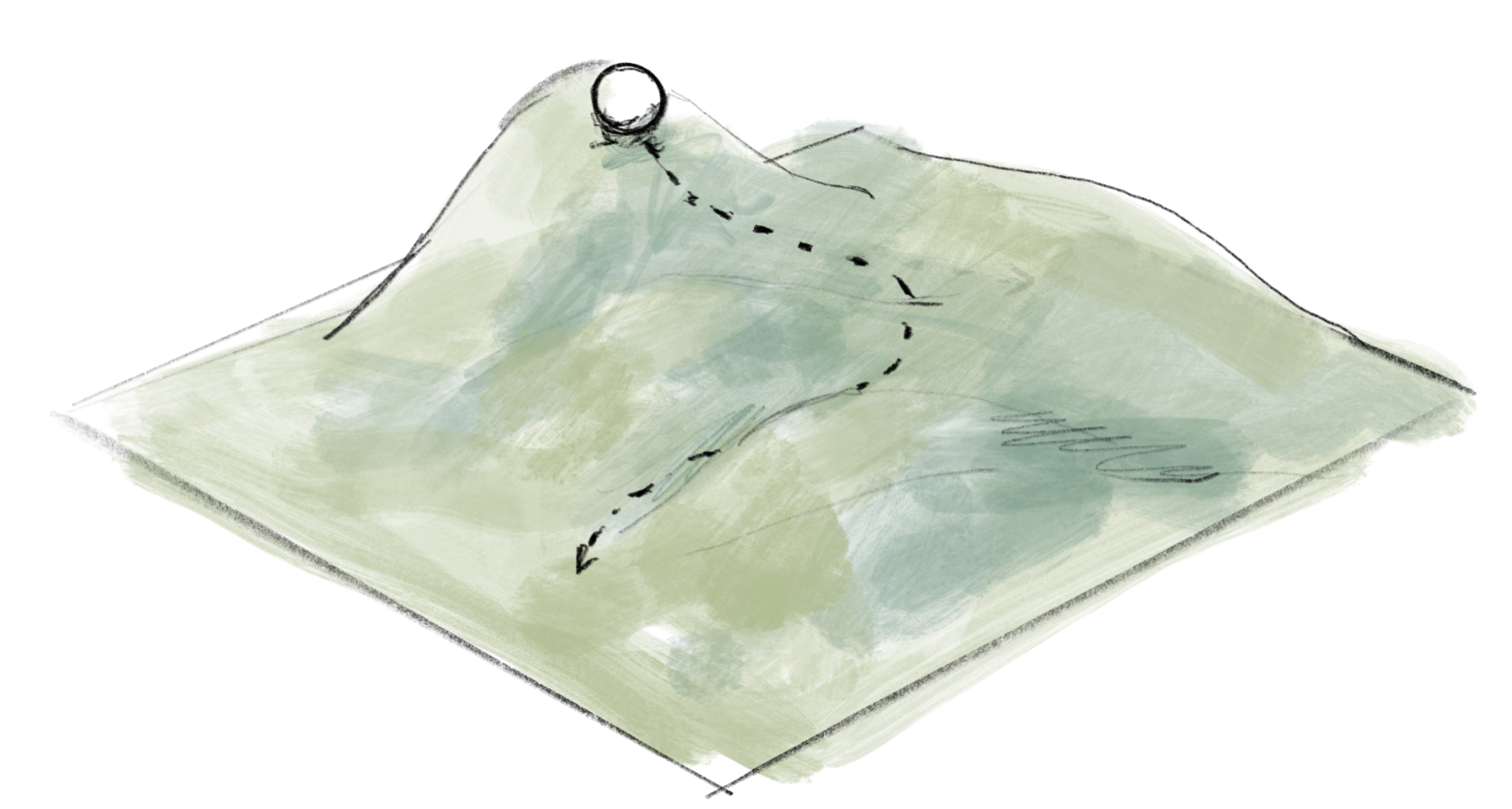
We use the term “gradient” to refer to a vector that indicates the direction of the greatest rate of increase of a function, with its magnitude representing the rate of increase in that direction. For instance, in the case of room temperature, the gradient points to the direction in which the temperature will increase the most, with its magnitude indicating how fast it will increase. Similarly, on a hill, the gradient points to the steepest path from where you stand, with its magnitude representing the steepness of that path. Using this concept, the answers to both questions above are equal to the “opposite of the gradient at the given point”.
関数の値が最も大きく変化する向きを示すベクトルを「勾配 (gradient) 」と呼び、その大きさは向きにおける変化する速さを表します。例えば、室温の場合、勾配は温度が最も上昇する方向を指し、その大きさは上昇速度を示します。丘の上では、勾配は立っている場所から最も険しい道を指し、その大きさはその道の険しさを表します。この概念を使うと、上の質問の答えは両方とも「与えられた点での勾配の反対」になります。
Gradient of a function is often denoted as (nabla), or and is given by:
関数の勾配は、しばしば(ナブラ)またはと表記され、次のように定義されます。
So gradient in fact is a vector made of the rate of change, or the derivatives of each variable combined together.
つまり勾配は、それぞれの変数の微分を結合してベクトルにしたものです。
As you can see from these examples of temperature and height on a hill, the distribution and changes of a value are typically very arbitrary and cannot be represented by a formula. So, gradients in computer simulations are usually calculated with numerical differentiation.
丘の高さや温度や例からわかるように、値の分布や変化は大抵かなりランダムで、数式で表すことができません。そのため、コンピュータシミュレーションにおける勾配は通常、数値微分によって計算されます。
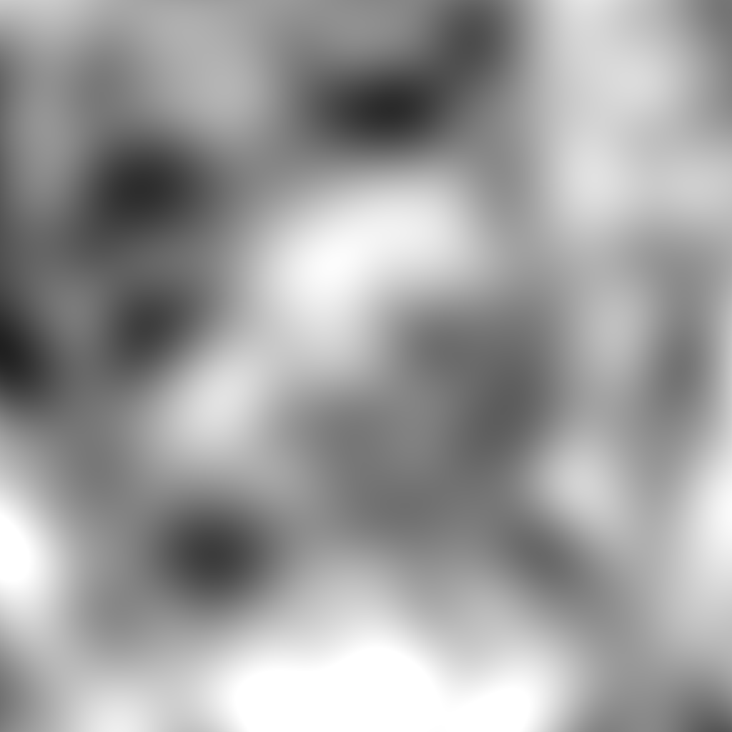
Think about a terrain’s height, often represented as a “height map”, a 2D array that stores the height of each point in a grid. A height map can look like this: the whiter the cell, the higher the value, indicating a higher position.
ある地形の高さについて考えてみましょう。凹凸の高さはハイトマップと呼ばれる、グリッド内の各点の高さを格納する2次元配列で表されます。下はハイトマップの例です。白いセルほど値が高く、高い位置を示します。
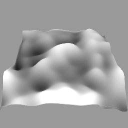
左のハイトマップを3Dレンダリングしたもの
To obtain a gradient of a cell, we can just compare the values of neighboring cells.
あるセルの勾配を計算するには、単純に隣り合うセルの値を比較します。
To obtain the derivative along the rows, compare the value of the cell to the right and left, and divide the difference by the distance.
行方向の勾配を得るには右側のセルの値と左側のセルとの差を求めて、その差を距離で割ります。
Similarly for along the columns:
列方向も同様です。
In the demo below, the grid on the left is the height map, and the arrows to the right represent the gradient.
下のデモの左側はハイトマップを、右側はその勾配を矢印で表したものです。
The concept of the gradient is very useful in simulating many real-world phenomena and plays a crucial role in AI algorithms. Most AI algorithms are based on huge multivariable functions with a crazy number of parameters. The gradient is used to gradually optimize these parameters by finding the best direction to reduce errors.
勾配の概念は、多くの現実世界の現象をシミュレートするのに非常に便利で、またAIのアルゴリズムにおいても重要な役割を果たしています。ほとんどのAIアルゴリズムは、膨大な数のパラメータを持った巨大な多変数関数に基づいています。勾配は、答えの間違いを減らすための最適な方向を見つけて、これらのパラメータを徐々に最適化するために使われます。