Sound visualization 音の視覚化

“Audio-visual” is a cliché in visual coding and is still popular. By taking a sound source or input and analyzing the data, you can create various visual (and other) representations, ranging from practical visualizations to more expressive pieces. On this page, we will take a look at the fundamental structure of sound and examples of how to transform it into visuals.

「オーディオ・ビジュアル」は、コードでビジュアルを作る界隈では使い古されていながらも、今も人気のトピックです。音源、または音の入力を取り込み、データを分析することで、実用的なものからより表現豊かな作品まで、さまざまな視覚表現（およびその他の表現）を作り出せます。このページでは、音の基本的な構造とそれをビジュアルに変換する方法を見ていきます。

We will use the Web Audio API to play sound and get data for visualization. For more details about the Web Audio API, refer to this MDN page. You could also use p5.sound, which is a wrapper for the Web Audio API.
音の再生と可視化のためのデータ取得にWeb Audio APIを使用します。Web Audio APIの詳細については、MDNのページを参照してください。Web Audio APIをラップしたp5.soundを使うこともできます。

Characteristics of sound waves

音波の特性

Sound is a wave. It starts from an object, anything from a guitar string, vocal cords, a propeller, to an popping balloon. When an object vibrates, has repetitive motion, or causes some impact, it causes the particles of the medium around it to vibrate, transferring the vibrations from one particle to the next. In air, these vibrations manifest as fluctuating air pressure; in water and solids, the particles oscillate back and forth.

音は波です。この波はギターの弦、声帯、プロペラ、または破裂する風船など、あらゆる物体から始まります。物体が振動したり、ある動きを繰り返したり、衝撃を発生させると、その周りの媒体の粒子が振動し、振動は次の粒子へと伝わっていきます。空気中では、これらの振動は気圧の変動として現れます。水や固体では、粒子は前後に振動します。

When a sound wave reaches our ears, it causes our eardrums to vibrate. These vibrations are then translated into electrical signals in the inner ear, which the brain interprets as sound. It is fascinating, as we will see, the sound wave is just a messy up-down of the pressure level. But, we can hear different pitches and harmonies, and distinguish between various instruments, human voices, and different kinds of noise.

耳に音波が届くと、鼓膜が振動します。その振動は内耳で電気信号に変換され、脳はそれを音として解釈します。音波は雑然とした圧力レベルの上下動ですが、人がそこから異なる音の高さや調和、さらには様々な楽器や人の声、さまざまな種類の雑音を聞き分けられるのは驚異的なことです。

The characteristics of sound waves, such as frequency and amplitude, determine how we perceive different sounds. The frequency of a wave, measured in hertz (Hz), determines the pitch of the sound: higher frequencies produce higher-pitched sounds, and lower frequencies result in lower-pitched sounds. Meanwhile, the amplitude, or the height of the wave, determines the volume; larger amplitudes make louder sounds.

周波数と振幅などの音波の特性によって人がどのように異なる音を知覚するかが決まります。ヘルツ（Hz）で測られる波の周波数は、音の高さを決めます。周波数が高いほど音が高くなり、周波数が低いほど低音になります。一方で、振幅または波の高さは音量に関わり、振幅が大きいほど、より大きな音になります。

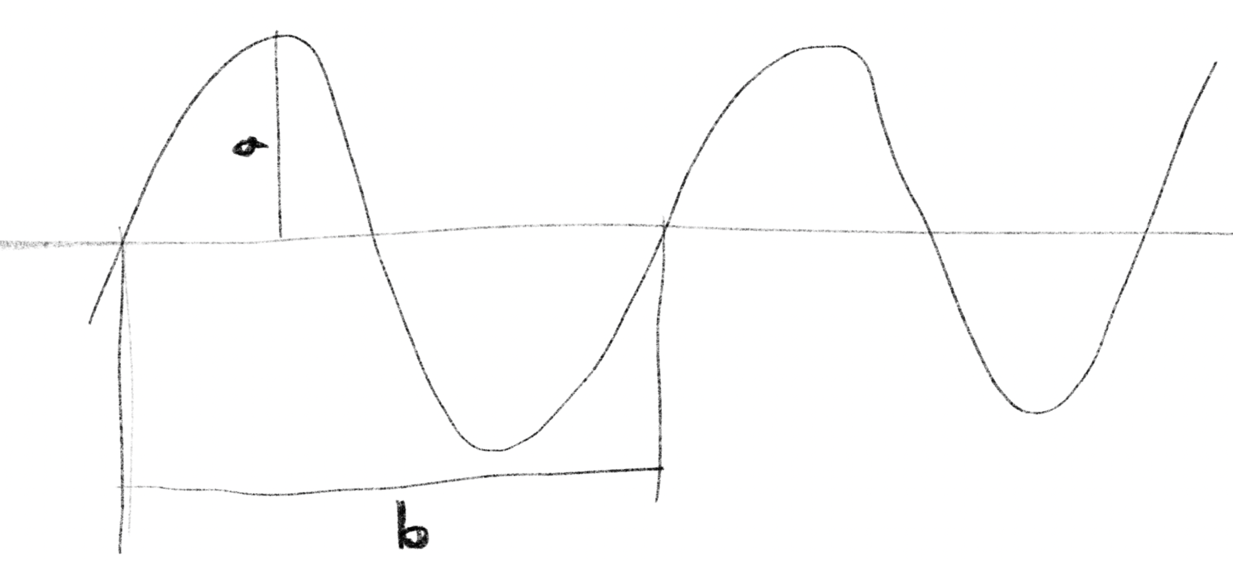
In this picture, the maximum height of the wave, $a$ in the figure, is the amplitude, and the length of $b$ is the wavelength. Or if the horizontal axis of the graph is time, $b$ is the period, which is the time it takes for each oscillation. Frequency is the number of oscillations per second, which is one second divided by the period, $f = 1 /T$, where $T$ represents the period.

図の$a$、波の最大の振れ幅が振幅（amplitude）、$b$の長さが波長（wavelength）です。横軸が時間であれば$b$は1回の振動にかかる時間、周期（period）になります。1秒間の振動の回数が周波数（frequency）で、周期をTとすると、これは1秒を周期で割ったもの $f = 1 / T$ になります。

Sound wave as digital data

デジタルデータとしての音波

In a digital medium, a sound wave is represented as an array of numbers that indicate the pressure at each moment. These numbers are referred to as “samples.” The quality and accuracy of the data depend on two main factors: the sampling rate and the bit depth. The sampling rate is the number of samples taken per second, and the bit depth determines the resolution of each sample. For example a standard CD uses a sampling rate of 44,100 Hz (or 44.1 kHz) and a bit depth of 16 bits. This means that 44,100 samples are captured per second, and each sample is a 16-bit number. These standards are designed to capture frequencies within the human hearing range (approximately 20-20,000 Hz) and provide sufficient dynamic range (the difference between the quietest and loudest sounds). Although CDs are considered outdated, these standards are still used as a reference, although there are formats with higher fidelity such as 32-bit audio.

デジタルの媒体では、音波は瞬間ごとの圧力を示す数値の配列として表現されます。これらの数値は「サンプル」と呼ばれます。データの品質と精度は主に、サンプリングレートとビット深度という2つ要素に依存します。サンプリングレートは1秒あたりのサンプル数を示し、ビット深度は各サンプルの解像度を決定します。たとえば、標準的なCDではサンプリングレート44,100 Hz（または44.1 kHz）、ビット深度16ビット、つまり、1秒あたりに44,100のサンプルが記録され、それぞれのサンプルは16ビットの数値で表されます。これらの標準は、人間の聴覚範囲（約20〜20,000 Hz）内の周波数を記録し、十分なダイナミックレンジ（最も静かな音と最も大きな音の差）を提供できるように設計されています。CDはもう現役を去りつつありますが、これらの標準は今も参照されています。他にも、32ビットオーディオなど、より高い再現性を持つフォーマットも存在します。

On browsers, the Web Audio API provides a node called AnalyserNode that lets us to read real-time information about the currently playing sound. With its getFloatTimeDomainData() method, you can read the sound wave into a Float32Array. Each value is normalized between -1 and 1.

ブラウザ上では、Web Audio APIが提供するAnalyserNode というノードを使って再生中の音に関する情報をリアルタイムに読み取ることができます。getFloatTimeDomainData() メソッドを使用すると、音の波形をFloat32Arrayに読み取ることができます。各値は-1から1の範囲で正規化されています。

The demo below creates sounds (sine waves) of different frequencies and amplitudes and uses the API to visualize the data as a graph. Notice how the shape of the graph is related to the sound you hear. You can click on the canvas to turn the sound on or off.

下のデモでは、異なる周波数と振幅の音（正弦波）を生成し、このAPIを使ってデータをグラフとして表示します。グラフの形と聞こえる音の関係に注目してください。キャンバスをクリックすると音をオン・オフすることができます。

Adjust your volume before starting the sound.
再生する前にボリュームを調整しておきましょう。

The sounds we hear in real life are not as simple as sine waves. The example below plays several (digital) instruments one by one, and then all together at the end. Notice that each instrument has a unique wave shape. When played together, these waveforms are added up to form a more complex shape, but you can still somewhat see the characteristics of the instruments. Also, these instruments have clear repetition in their waveforms, which lets us perceive the pitch of the notes.

実生活で耳にする音は、正弦波ほど単純ではありません。下の例では、いくつかの（デジタル）楽器を順番に演奏し、最後に全部合わせて鳴らします。それぞれの楽器には独自の波形があります。重ねて演奏すると、これらの波形は足し合わされてより複雑な形状になりますが、それでもまだ楽器の特性が見て取れます。また、これらの楽器の波形には明確な繰り返しがあり、音の高さを知覚することができます。

The next recording plays street noise with several men shouting. The waveform looks much more random, finely grained, and lacks a clear pitch. You can still see that the amplitude corresponds to the loudness of the sound you hear.

次の録音では、通りの騒音と数人の男性が大声を出す様子が聞こえます。波形はより細かくランダムで、明確な音の高さがありませんが、振幅が音の大きさに対応していることは見て取れます。

The sound data is simply an array of numbers, which can be applied to anything, such as colors, positions, shapes, etc. The demo below uses these values to modify the hue, brightness, and vertical length of lines. Just a few changes in the draw() function can create a completely different appearance.

音声データは単に数値の配列なので、色、位置、形状など何にでも適用することができます。以下のデモでは、これらの値を使って、線の色相、明度、垂直方向の長さを変化させています。draw() 関数をちょっと書き換えるだけで、まったく異なる見た目が作り出せます。

Loudness

音の大きさ

Depending on your objectives or the insights you seek from the data, the raw sound data can be too detailed and granular. For example, if your goal is to visualize a voice recording to distinguish the speech segments and pauses, you may want some aggregated data that reflect the overall loudness of the sound over time.

使用目的やデータから知りたい内容によっては、生の音声データでは細かすぎる場合があります。たとえば、音声録音をビジュアライズして発話部分と休止部分を見分けたい場合、時間の経過に対する音の大きさの変化を示すまとまったデータが欲しくなるでしょう。

A common method for calculating the loudness of a sound over a specific time period is to use the RMS (Root Mean Square). As mentioned before, each sample value ranges from -1 to +1, so simply taking the average would yield a value close to zero. Instead, the RMS method squares each sample value, which turns all values positive. Then, it averages these squared values and finally calculates the square root of this average.

特定の時間帯における音の大きさを計算するには、RMS（2乗平均平方根）が一般的に用いられます。前述の通り各サンプル値は-1から+1の範囲にあるので、単純に平均を取ると値はほぼゼロになってしまいます。RMSでは各サンプルの値を2乗しすることで全ての値を正に変換した後で平均を求め、その平均の平方根を求めます。

$\begin{aligned} \text{RMS} = \sqrt{\frac{1}{N} \sum_{i=1}^{N} x_i^2} \end{aligned}$

$N$ is the number of samples

$x_i$ represents each individual sample value

$N$ はサンプルの数

$x_i$ はそれぞれのサンプル値を示す。

Not only does it address the negative values, but the square of the values better corresponds to the power of the sound waves, which is the energy transferred by the wave in a given time.

この方法だと負の値に対応できるだけでなく、値の2乗は音波の「パワー」、つまり音が一定の時間内に伝達するエネルギーをよりよく表しています。

The demo below calculates the RMS value for each frame, stores them in an array, and visualizes them as a bar chart. This visualization provides a better overview of the sound data over much longer period of time compared to the raw wave form (It also looks like a background for an old school 2D shooting game, which is cool).

下のデモでは、フレームごとにRMSを計算して配列に保存し、棒グラフとして表示します。この方法では、生の波形と比較して、長時間にわたる音データの概要をうまく示すことができます（昔ながらの2Dシューティングゲームの背景みたいで格好良い感じもあります）。

Of course, you can get data separately for each left and right channel. Here, I have applied some feedback techniques we discussed in Pencil, Brush and Paint to the graphics.

もちろん、左チャンネルと右チャンネルのデータを個別に取得することもできます。ここでは、Pencil, Brush and Paintで見たフィードバックの手法をグラフィックに適用しました。

Fast Fourier transform

高速フーリエ変換

In the previous section, we summarized raw sound data into a single value (or two if you separate left and right channel values) that represents the loudness at the moment. In this section, we will use an algorithm called Fast Fourier Transformation (FFT) to analyze the sound data as a spectrum.

前のセクションでは、生の音データを1つの値（左右のチャンネルで値を分ける場合は2つ）にまとめて、その瞬間の音の大きさを表しました。このセクションでは、高速フーリエ変換（FFT）と呼ばれるアルゴリズムを使用して、音データをスペクトルとして解析します。

As discussed on the Fourier series page, a periodic wave, which has a repeating pattern, can be decomposed into a series of sine waves with different frequencies. The Fourier Transform extends this concept to non-periodic waves or functions (you can think of sound as a function that takes time as input and returns a value). While the Fourier series returns discrete sine waves, the Fourier Transform generates a continuous function that provides the phase and amplitude of a sine wave for any given frequency. In other words, with the Fourier transform, you can investigate the amount of different frequency components that the sound has at a given moment. (For example, does it have more low bass sound or treble sound?)

フーリエ級数のページで見たように、繰り返しのパターンを持つ周期的な波は、異なる周波数を持つサイン波の級数として分解できます。フーリエ変換は、この概念を非周期的な波や関数に拡張します（音は時間を入力として値を返す関数と考えられます）。フーリエ級数は離散的なサイン波を返しますが、フーリエ変換は、任意の周波数に対してサイン波の位相と振幅を返す連続関数を生成します。言い換えると、フーリエ変換を使うと、音がある瞬間に異なる周波数成分をどれだけ含んでいるかを調べることができます（例えば低音や高音のどちらが多いのか調べることができます）。

The relationship between Fourier series and Fourier transform is like the distinction between integers and real numbers. Also, the spectrum of frequency you get from the Fourier transform is analogous to the spectrum of light. In fact, we use the term “white noise” to refer to noise that contains all frequency components equally. This term came from the fact that light that contains all visible frequency components appears white.

フーリエ級数とフーリエ変換の関係は、整数と実数の違いに例えられます。また、フーリエ変換から得られる周波数のスペクトルは、光のスペクトルにも似ています。実際、「ホワイトノイズ」とは全ての周波数成分を等しく含むノイズを指しますが、この用語は、全ての可視周波数成分を含む光が白く見えるという観察に由来しています。

Fast Fourier transform (FFT) is a practical implementation of the Fourier transform. It takes sound data (or a function) as input and returns an array of numbers that represent different frequency components. It is probably easier to see it in action. In the demo below, the FFT is used to generate an array for 256 frequency bands. The number of bands (often called “bins” too) is specified in the line analyser.fftSize = 256. The level of each frequency is obtained with analyser.getFloatFrequencyData(dataArray). Each frame, a bar graph is drawn to visualize the frequency components. The bars on the left represent low-frequency components, while the bars on the right represent high-frequency components. See if this corresponds to what you hear.

高速フーリエ変換（FFT）は、フーリエ変換を実用的に実装した物です。音データ（または関数）を入力として受け取り、異なる周波数成分を表す数値の配列を返します。多分実際に見た方が簡単でしょう。下のデモではFFTを使って256の周波数帯の配列を生成しています。周波数帯の数（英語ではこの帯をband、またはbinと呼びます）は、analyser.fftSize = 256の行で指定されています。各周波数のレベルはanalyser.getFloatFrequencyData(dataArray)で取得し、フレームごとに周波数成分を表す棒グラフが描かれます。左側のバーは低周波数成分を、右側のバーは高周波数成分を表しています。聞こえる内容に対応して見えるでしょうか。

The actual size of the array you get will be half of the number you specified with the analyser.fftSize. Let me skip explaining why because it requires delving deep into the math of the Fourier transform.
実際の配列のサイズは、analyser.fftSize で指定した数値の半分になります。理由の説明はフーリエ変換の数学に深く立ち入る必要があるのでスキップします。

Once we have these values, we can use them in any way. Here is an example of slicing and adding a glitchy effect to a portrait of a somber Dutch monk, making him shake his head to the music.

一度値が手に入れば、自由に使うことができます。下の例では厳格なオランダ修道僧の肖像画を切り分け、壊れたようなエフェクトをかけ音楽に合わせて頭を振らせています。

To explore further

さらなる探求

We have explored various methods of capturing sound as data and using that data to create visual representations. In a real project, you may want to combine these with other types of ideas or find unique uses for the data, as relying solely on sound synchronization can appear a bit overdone. But first and most importantly, just have fun sketching!

このページでは音をデータとして扱い、視覚的な表現を作る様々な方法を見てきました。実際のプロジェクトでは、音の同期だけに頼るとありきたりな印象になることもあるので、他のタイプのアイデアと組み合わせたり、ユニークなデータの使い方を見つけると良いかもしれません。何はともあれ、まずは楽しみながらスケッチしましょう。

We have discussed the characteristics of sound as a wave in the Wave pages as well.

音の波としての特性については波のページでも取り上げています。

If you are interested in the implementation of FFT, the FFT page on the Algorithm Archive can be a good starting point.

もしFFTの実装に興味があれば、Algorithm ArchiveのFFTのページが出発点として良いかもしれません。

For more a friendly yet thorough introduction to Fourier transform, I recommend “Who Is Fourier?: A Mathematical Adventure” by Transnational College.

より親しみやすく、かつ詳細なフーリエ変換の入門としては、Transnational Collegeの「Who Is Fourier?: A Mathematical Adventure」がお勧めです。日本語版もあります。