Neural Network ニューラルネットワーク

Neural networks are essential to AI technologies today, from classic image classifiers to the latest large language models. On this page, we’ll explore the foundation of their mechanism. Since there are already many great articles and books on this topic, we’ll focus on building intuition with simple examples while glossing over details.

ニューラルネットワークは、クラシックな画像分類器から最新の大規模言語モデルまで、現代のAI技術には欠かせません。このページではその仕組みの基礎について見ていきます。この分野にはもうたくさんの優れた記事や書籍があるので、詳細は飛ばしてシンプルな例で直感的な理解を目指します。

So what is a neural network? You probably know it’s inspired by the human brain, but it’s not really a simulation of one. No matter how sophisticated they look from the outside, neural networks do one thing—they create a mathematical function that takes an input and produces the corresponding output.

ニューラルネットワークとは何でしょうか。人間の脳から着想を得ていることは知られていますが、実際には脳のシミュレーションではありません。どれだけ洗練されているように見えても、ニューラルネットワークがすることは1つで、入力を受け取り対応する出力を生成する、数学的な関数を作ることです。

$\text{Input} \implies \boxed{\text{ \textbf{Function} }} \implies \text{Output}$

For example, say you want a model that can tell if there’s a cat in a picture. That may not sound like a mathematical function, but it can be written as a function that takes all the RGB values of the pixels and returns a binary (yes or no) or the probability of a cat’s presence.

例えば、画像に猫が写っているかを判定するモデルが欲しいとします。数学的な関数とは思えないかもしれませんが、すべてのピクセルのRGB値を入力として受け取り、バイナリ（はい、いいえ）か、猫がいる確率を返す関数として記述できます。

The problem here is that no one knows how to write such an algorithm, but a well-designed neural network with enough examples of images with and without cats can forge a function by nudging a lot of numbers inside while reacting to these examples.

ここで問題なのは、そんなアルゴリズムの書き方は誰にもわからないことですが、適切に設計されたニューラルネットワークは、十分な数の猫ありと猫なしの画像があれば、それらの例に応じて内部の数値を調整し、関数を構築できます。

Being a mathematical function means the output is uniquely determined for a given input. People often say AI is unpredictable, but neural networks are completely deterministic. If a model returns different results every time, it’s because it’s intentionally programmed to use random input behind the scenes.

数学的関数であるというのは、入力が決まれば出力も一意に決まるということです。AIは予測不可能だとよく言われますが、ニューラルネットワークは完全に決定論的です。モデルが毎回違う結果を返すなら、それは意図的に裏でランダムな入力を使うようプログラムされているからです。

Neuron

ニューロン

Neural network is built on an incredibly simple math formula, something that looks like:

ニューラルネットワークは、下のような、びっくりするほどシンプルな数式からできています。

$y = \max(0, x \cdot w + b)$

If $x = 0.2$ , $w = 2$ , $b = 0.3$ , then it’s $max(0, 0.2 \times 2 + 0.3) = 0.7$ . Easy, right? This is our neuron. $x$ is the input, $w$ is called weight and $b$ is bias, $y$ is the output. The only complication here is that a neuron usually takes multiple inputs, so the $x, w$ are vectors. So it would look like this.

、 $w = 2$ 、 $b = 0.3$ なら、 $max(0, 0.2 \times 2 + 0.3) = 0.7$ です。簡単ですね。これがニューロンです。 $x$ は入力、 $w$ は重み（weight）、 $b$ はバイアス（bias）、 $y$ は出力を表します。ただひとつ複雑なのは、ニューロンは大抵、複数の入力を受け取ることです。すると $x, w$ はベクトルになるので、次のようになります。

$y = \max(0, \mathbf{x} \cdot \mathbf{w} + b)$

$y = \max(0, \begin{bmatrix} 0.8 & 0.1 \end{bmatrix} \cdot \begin{bmatrix} 1.2 \ -0.5 \end{bmatrix} - 0.2) = 0.71$

Let’s see what this function actually does. In the demo below, the position in the grid represents two values in the input $\mathbf{x}$ . $\mathbf{w}$ and $b$ are fixed to the numbers above ( $\begin{bmatrix} 1.2 \ -0.5 \end{bmatrix}$ and $- 0.2$ ). The height of the line represents the output $y$ , which makes a nice slope on the plane.

この関数が実際に何をするのか見てみましょう。下のデモでは、グリッド上の位置が入力 $\mathbf{x}$ の2つの値を表します。 $\mathbf{w}$ と $b$ は上の数値（ $\begin{bmatrix} 1.2 \ -0.5 \end{bmatrix}$ と $- 0.2$ ）に固定されています。線の高さは出力 $y$ を表し、平面上にきれいな傾斜を描いています。

Let’s add one more neuron to the mix. The demo below shows two of the same neuron with different parameters ( $\mathbf{w}$ and $b$ ) merged together. You can imagine that adding more neurons allows us to create much more complex shapes.

もう1つニューロンを足してみましょう。下のデモでは、パラメータ（ $\mathbf{w}$ と $b$ ）だけが異なる同じニューロンを2つ組み合わせています。ニューロンを増やせば、より複雑な形を作れることが想像できるでしょう。

In fact, the essence of a neural network is connecting many simple functions like this and letting the model find the right parameters to approximate the function we want.

実際、ニューラルネットワークの本質は、このようなシンプルな関数をたくさん繋げて、モデルに適切なパラメータを見つけさせ、望む関数を近似させることにあります。

In this example, we used a 2D vector as input so that we can visualize the function, but the input can be very high-dimensional, like 512, or 1,024, or a lot more. It is really hard to imagine such a high-dimensional world, but the basics are the same. Based on the input—no matter how big the vector size is—each neuron will output a value.

この例では可視化のために2次元ベクトルを入力として使いましたが、実際の入力はとても高次元、例えば512次元、1024次元や、それ以上になることもあります。そんな高次元の空間を思い浮かべるのは厳しいですが基本は同じで、ベクトルのサイズに関わらず、それぞれのニューロンは入力に基づいて値をひとつ出力します。

Activation Functions

活性化関数

In the formula above, the $max(0, …)$ is critical. In the demos, you noticed that the neuron’s output is bent—there’s a slope and then a flat part. Without this bending, each neuron’s output would be linear, just a slanted plane. Linear functions are problematic because adding multiple linear functions still gives you a linear result. This means you can’t create any complex shapes.

上の式の $max(0, …)$ はとても重要です。デモで気づいたと思いますが、ニューロンの出力には傾斜した部分と平らな部分があり、折れ曲がっています。この折れ曲がりがないと、それぞれのニューロンの出力は線形な、ただ1枚の傾いた平面になります。線形関数には問題があって、複数足し合わせても結果はやはり線形になるので、複雑な形を作ることができません。

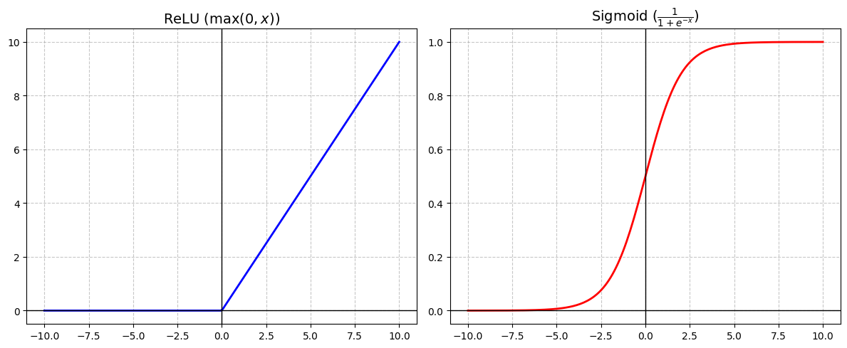
Several functions called activation functions are commonly used in neural networks to create non-linearity. The one above that uses $max$ is called ReLU (Rectified Linear Unit). Another, shown below, is the Sigmoid function. Sigmoid was once very popular for its smooth S-curve, but ReLU has become more common in recent models.

ニューラルネットワークで非線形性を生み出すには、活性化関数と呼ばれる関数がいくつかあります。上の $max$ を使うものは ReLU（Rectified Linear Unit、正規化線形ユニット）と呼ばれます。下に示したもう1つはシグモイド関数です。滑らかなS字曲線を描くシグモイド関数はよく使われていましたが、最近のモデルでは ReLU の方が一般的です。

Google Colab

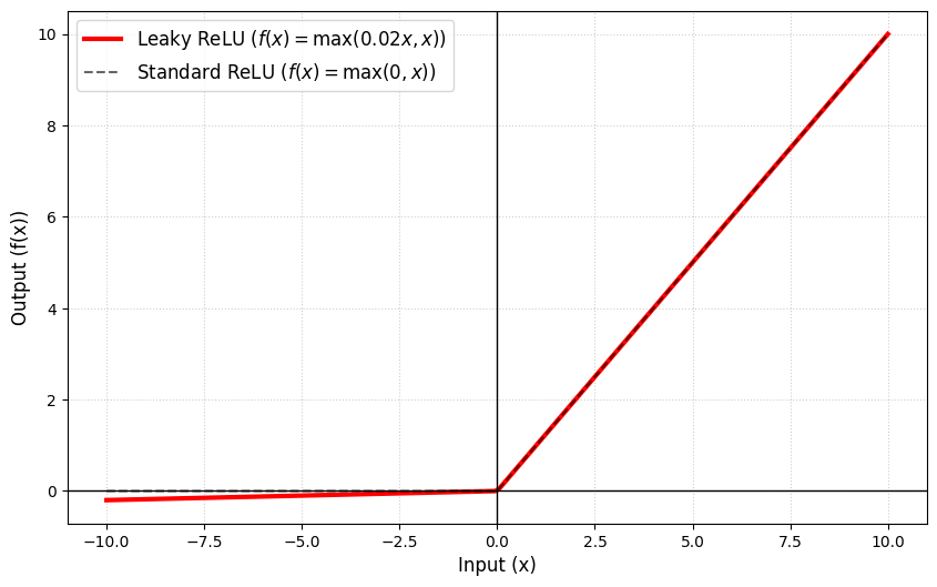
In the demos below, we will use a variation called leaky ReLU. It is very similar to ReLU but with a slight, non-zero slope for negative inputs ( $\alpha$ in the formula is a small number, such as 0.01). This helps a lot in the training process that we’ll discuss below.

下のデモでは、leaky ReLU というバリエーションを使います。ReLU とよく似ていますが、負の入力に対してゼロではない、わずかな傾きを持ちます。式の中の $\alpha$ は 0.01 などの小さな数値で、これは後で説明するトレーニングで大きく役立ちます。

$f(x) = \begin{cases} x & \text{if } x > 0 \ \alpha x & \text{if } x \le 0 \end{cases}$

Building a network

ネットワークを構築する

Now that we know how a neuron works, let’s connect some of them to make a network that can do something a little more interesting.

ニューロンの仕組みがわかったので、ニューロンをいくつか繋いで、もう少し面白いことができるネットワークを作ってみましょう。

We aim to detect whether a point on a 2D plane is inside a circle. For practical use, we don’t need a neural network for this. I’d even say we shouldn’t use one because a simple Pythagorean formula will give the perfectly correct answer, while neural networks won’t be perfect. But for our purpose, it’s a nice example that’s very easy to visualize.

2次元平面上の点が円の内側にあるか判定することを目指します。実用上は、ニューラルネットワークは必要ありません。単純なピタゴラスの定理で完璧に正しい答えが得られるのに対し、ニューラルネットワークでは完璧にならないため、むしろ使うべきではないとさえ言えます。ですが今回の目的には、視覚化しやすい良い例です。

The demo below implements this model in p5.js. The large circle in the middle is the target. The small circles represent the model’s predictions. Each circle’s size shows how confident the model is that the point is inside the target. A value of zero (or below) means the model thinks the point is definitely outside. The larger the value, the more likely it is inside. The circle size is proportional to this value, and circles turn black when the value reaches 0.5.

下のデモは、このモデルを p5.js で実装しています。真ん中の大きな円がターゲットで、小さな円はモデルの予測を表します。それぞれの円の大きさは、その点がターゲットの内側にあるとモデルがどれだけ確信しているかを示します。値がゼロ（またはそれ以下）なら、モデルはその点が確実に外側にあると考えています。値が大きいほど、内側にある可能性が高くなります。円のサイズはこの値に比例し、値が0.5に達すると黒くなります。

You can see the model starts with random predictions but gradually learns to approximate the shape much better (though it won’t be perfect). Click the canvas to reset the model and randomize all the parameters. Try it several times.

モデルは最初ランダムな予測から始まりますが、（完璧にはなりませんが）徐々に形をより正確に近似するように学習します。キャンバスをクリックするとモデルがリセットされ、すべてのパラメータがランダム化されます。何度か試してみましょう。

Model Structure

モデルの構造

The model looks like the diagram below. Two circles in the input represent the x and y position. These two inputs go through eight neurons similar to the ones we looked at above, but with leaky ReLU. $\mathbf{p} = [x, y]$ . $j$ is an index for each of our 8 neurons.

モデルを下の図に示します。入力の2つの円はxとyの位置を表します。この2つの入力は、先ほど見たものと似ていますがleaky ReLUを使う8つのニューロンを通ります。 $\mathbf{p} = [x, y]$ で、 $j$ は8つのニューロンそれぞれのインデックスです。

$\text{h}$

This layer of 8 neurons is called a hidden layer because it’s hidden in the middle of the network.

この8つのニューロンからなるレイヤーはネットワークの中間に隠れているので、隠れ層と呼ばれます。

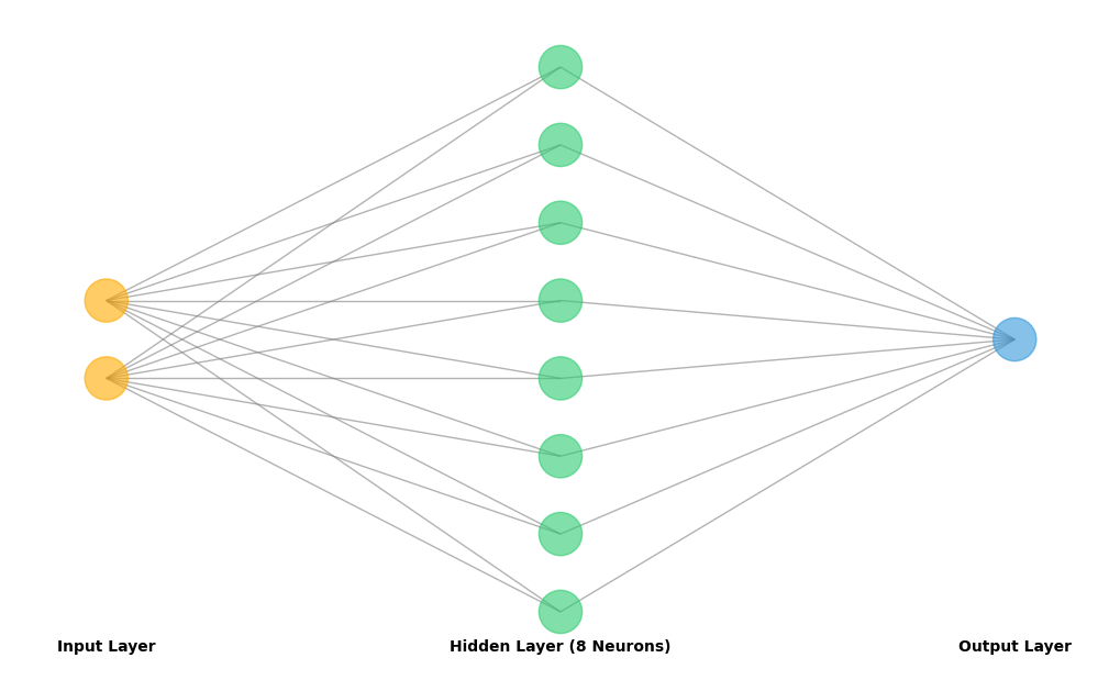
The final output layer takes all the outputs from the 8 neurons ( $\mathbf{h} = [h_1, h_2, \dots, h_8]$ ), merges them by multiplying with another set of weights and adding a bias, then applies the activation function. We could use the Sigmoid function to constrain the output to the range (0, 1), but for simplicity, let’s use the same approach everywhere.

最後の出力層は、8つのニューロンすべての出力（ $\mathbf{h} = [h_1, h_2, \dots, h_8]$ ）を受け取ります。それらに別の重みをかけ、バイアスを足し合わせた後、活性化関数を適用します。出力を(0, 1)の範囲に制約するにはシグモイド関数を使うこともできますが、シンプルにするため、すべての層で同じアプローチを使いましょう。

$\text{output} = \text{leakyReLU} \left( \mathbf{h} \cdot \mathbf{w}_2 + b_2 \right)$

As you can see in the demo, 8 neurons aren’t enough to make a perfect circle, but they’re sufficient for this small experiment. Remember the first visualization. Each neuron can only create a simple folded shape, and 8 of them can only make an octagon. The more neurons you add, the more complex and nuanced shapes you can create. However, adding too many can slow down training and reduce performance.

$\text{output} = \text{leakyReLU} \left( \mathbf{h} \cdot \mathbf{w}_2 + b_2 \right)$

デモで見てわかるように、8つのニューロンでは完璧な円を作るには足りませんが、この小さな実験には十分でしょう。最初のビジュアライゼーションを思い出してください。それぞれのニューロンはシンプルな折れ曲がった形しか作れないので、8つでは八角形しか作れません。ニューロンを増やせば増やすほど、より複雑で繊細な形を作ることができますが、増やしすぎるとトレーニングが遅くなったり、性能が落ちることもあります。

Training

トレーニング

Now we have a network, but it won’t produce anything close to a correct answer because the weights and biases aren’t configured properly yet.

これでネットワークができましたが、重みとバイアスがまだ適切に設定されていないため、正しい答えのようなものは何も出力されません。

The process we’re going to use to set up these parameters is called supervised learning, which involves showing a bunch of examples of input and output.

これらのパラメータを設定するには、入力と出力の例をたくさん見せる、教師あり学習と呼ばれるプロセスを用います。

For real products, we need to gather a large dataset of real-life examples, like a lot of photos for the cat detector. But for this particular example, we deliberately chose a question we know the answer to. So we can write code to randomly pick a point and use the Pythagorean theorem to label it with the correct answer: 0 for outside, 1 for inside.

実際の製品では、猫検出器用の大量の写真のように、現実の例を集めた大規模なデータセットが必要です。しかし今回の例では、わざと答えがわかっている問題を選びました。そのため、ランダムに点を選び、ピタゴラスの定理を使って正しい答え（外側なら0、内側なら1）でラベル付けするコードを書くことができます。

At the start of training, we set all the parameters to random values. The training process is then a loop of the following steps:

トレーニングの開始時には、すべてのパラメータをランダムな値に設定します。トレーニングのプロセスは、下記のステップの繰り返しです。

Forward Pass

フォワードパス

We give the model an input - a random point $\mathbf{p}$ and see what it predicts.

モデルにランダムな点 $\mathbf{p}$ を入力として与え、何を予測するかを見ます。

Error

誤差

We compare the model’s prediction to the correct answer(the Pythagorean formula), and calculate the error - how off the predictions is from the target. The error value is simply the difference between the model’s prediction and the target.

モデルの予測を正しい答え（ピタゴラスの定理）と比較し、誤差、つまり予測がターゲットからどれだけずれているかを示す値を計算します。誤差の値は単純に、モデルの予測とターゲットの差です。

$\text{Error} = \text{prediction} - \text{target}$

Backpropagation

バックプロパゲーション

This is where the magic happens. We work backward from the end of the network to figure out how much each weight and bias contributed to the error. Then we nudge them slightly in the right direction.

ここが秘訣です。ネットワークの終わりから逆向きに計算し、それぞれの重みとバイアスが誤差に対してどれだけ影響したかを調べ、値を正しい方向へ少しずつ調整します。

I recommend skipping to the code examples below and comparing them if these math notations throw you off.

数学的な表記で挫けそうな場合は、その下のコードの例に飛んでから比較することをお勧めします。

First, we calculate the responsibility for the error at each layer:

まず各レイヤーにおける、誤差に対する責任を計算します。

Output Layer : $\delta_{out} = (pred - t) \cdot \text{dAct}(outZ)$

Hidden Layer (Neuron $j$ ) : $\delta_{j} = (\delta_{out} \cdot w_{2,j}) \cdot \text{dAct}(h_{z,j})$

Here, $\text{dAct}$ is the derivative of the activation function (leaky ReLU), and $outZ$ is the output before applying the activation function. The derivative helps us find the right direction to nudge, showing how much the output would change if we adjusted $outZ$ slightly.

ここで、 $\text{dAct}$ は活性化関数（leaky ReLU）の微分、 $outZ$ は活性化関数を適用する前の出力です。微分は $outZ$ をわずかに変えた場合の出力の変化を示すことによって、調整の方向を教えてくれます。

Leaky ReLU is preferred over ReLU because it ensures the derivative never becomes zero, which would make the nudge amount zero.

Leaky ReLU が ReLU より好まれるのは、微分がゼロにならないことを保証してくれるからです。微分がゼロだと調整量もゼロになってしまいます。

Notice that the output layer’s responsibility ( $\delta_{out}$ ) is used to calculate each hidden neuron’s responsibility, multiplied by its weight and derivative. If there were more layers, each neuron’s value would feed into the previous layer. This is why it’s called backpropagation—the algorithm moves backward through the network from end to beginning, determining how much to adjust each parameter.

出力層の責任（ $\delta_{out}$ ）がそれぞれの隠れニューロンの責任を計算に使われ、その重みと微分が掛け合わされます。もっと多くのレイヤーがあれば、各ニューロンの値は前の層に伝播していきます。これが誤差逆伝播法と呼ばれる理由です。アルゴリズムはネットワークを終わりから始まりへ逆向きに進み、各パラメータの調整量を決定します。

Once we have those responsibility values, we apply the nudge.

責任の値が得られたら、調整を施します。

Output Layer

Weights ( $w_2$ ) : $w_{2,j} = w_{2,j} - \eta \times (\delta_{out} \times h_j)$
Bias ( $b_2$ ) : $b_2 = b_2 - \eta \times \delta_{out}$

Hidden Layer

Weights ( $w_1$ ) : $w_{1,j,\text{dim}} = w_{1,j,\text{dim}} - \eta \times (\delta_j \times p_{\text{dim}})$
Bias ( $b_1$ ) : $b_{1,j} = b_{1,j} - \eta \times \delta_j$

$\eta$ is a small number called the learning rate. it controls how much we adjust each parameter. If it’s too large, the weights jump around and never settle into a good range. If it’s too small, training takes forever.

$\eta$ は学習率と呼ばれる小さな数値で、それぞれパラメータの調整量を制御します。大きすぎると重みが飛び回って良い範囲に落ち着かず、小さすぎるとトレーニングが終わりません。

Code snippets

コードスニペット

Let’s look back the demo and try comparing the code with the explanation above.

デモを見直して、上の説明とコードを比較してみましょう。

The model object stores all the weights and biases.

modelオブジェクトはすべての重みとバイアスを格納します。

let model = {
  w1: [], b1: [], // Layer 1: 8 neurons, each with 2 weights and 1 bias
  w2: [], b2: 0   // Layer 2: 1 output neuron, combining the 8 signals
};

act() is the activation function (Leaky ReLU), and dAct() is the derivative of the activation function.

act() は活性化関数 (Leaky ReLU)で、dAct() は活性化関数の微分です。

function act(z) { return z > 0 ? z : z * 0.01; } // Leaky ReLU
function dAct(z) { return z > 0 ? 1 : 0.01; }

predict() and the first half of train() are the forward pass. This is where the model takes an input and guesses an output based on its current state. $train()$ has extra lines that randomly generate examples and capture each neuron’s output, but the underlying process is the same.

predict() と train() の前半がフォワードパスです。ここでモデルは入力を受け取り、現在の状態に基づいて出力を推測します。 $train()$ にはランダムな例を生成し、それぞれのニューロンの出力を記録する行が追加されていますが、基本的なプロセスは同じです。

function predict(nx, ny) {
	let h1_a = model.w1.map((w, i) => act(nx * w[0] + ny * w[1] + model.b1[i]));
	let outZ = model.b2;
	for (let i = 0; i < numHidden; i++) outZ += h1_a[i] * model.w2[i];
	return act(outZ);
}

function train() {
  for (let i = 0; i < trainingPerFrame; i++) {
    let nx = random(-1, 1);
    let ny = random(-1, 1);
    let target = sqrt(nx * nx + ny * ny) < 0.5 ? 1.0 : 0.0;

    // Forward
    let h1_z = [];
    let h1_a = [];
    for (let j = 0; j < numHidden; j++) {
      let z = nx * model.w1[j][0] + ny * model.w1[j][1] + model.b1[j];
      h1_z.push(z);
      h1_a.push(act(z));
    }

    let outZ = model.b2;
    for (let j = 0; j < numHidden; j++) {
      outZ += h1_a[j] * model.w2[j];
    }
    let prediction = act(outZ);
...

Then the latter half of train() is the backpropagation process. In the code, we represent the responsibility $\delta$ with variables like dOutZ and dZ. The learning rate $\eta$ is called learningRate.

そしてtrain()の後半がバックプロパゲーションのプロセスです。コードでは、責任 $\delta$ をdOutZやdZといった変数で表しています。学習率 $\eta$ はlearningRateです。

...
    // Backprop
    let error = prediction - target;
    let dOutZ = error * dAct(outZ);

    // Update Output Layer
    for (let j = 0; j < numHidden; j++) {
      let dW = dOutZ * h1_a[j];
      model.w2[j] -= learningRate * dW;
    }
    model.b2 -= learningRate * dOutZ;

    // Update Hidden Layer
    for (let j = 0; j < numHidden; j++) {
      let dH = dOutZ * model.w2[j];
      let dZ = dH * dAct(h1_z[j]);
      model.w1[j][0] -= learningRate * dZ * nx;
      model.w1[j][1] -= learningRate * dZ * ny;
      model.b1[j] -= learningRate * dZ;
    }
  }
}

Parameter Visualization

パラメータの可視化

The demo below shows the parameters from the model after successfully training. Because the model starts from a random state, the result will be different every time. Think of this as just one example.

下のデモでは、トレーニングが成功した後のモデルのパラメータを示しています。モデルはランダムな状態から始まり結果は毎回異なるので、これは1つの例として考えてください。

To avoid making it too cluttered, this demo fixes the $x$ input to zero and focuses only on $y$ . Move your mouse to change the $y$ input.

ごちゃごちゃしないように、このデモでは $x$ の入力をゼロに固定し、 $y$ だけに注目します。マウスを動かして $y$ の入力を変えてみましょう。

White circles represent outputs from the previous layer. Yellow boxes are the parameters $\text{w}$ and $b$ for each neuron. Move your mouse and watch how the input flows through these neurons. Notice how some neurons contribute more to the result than others? Those are the ones that learned to capture the y input better. Try modifying the code to see the effect of the $x$ input and compare.

白い円は前の層からの出力を表しています。黄色いボックスは各ニューロンのパラメータ $\text{w}$ と $b$ です。マウスを動かして、入力がこれらのニューロンを通ってどう流れるかを観察してください。他よりも結果に大きく貢献しているニューロンに気づいたでしょうか。それらは $y$ の入力をより上手く捉えるよう学習したニューロンです。コードを書き換え $x$ の効果も見て、比べてみましょう。

To learn more

さらに学ぶには

That’s it for this article. What we built above is fairly simple, but even the latest language models use basically the same networks—just with far more neurons and layers. Of course, there are various other tricks they use, but what we’ve seen here serves as their foundation.

この記事はここまでです。上で作ったものはかなりシンプルですが、最新の言語モデルでも、ニューロンと層がはるかに多いだけ基本的には同じネットワークを使っています。もちろん、他にも使われているテクニックは色々ありますが、それでも、ここで見たものが基盤となっています。

More practical networks usually have multiple layers that feed from one set of neurons to another before reaching the final output (along with other kinds of processes). The demo below shows how a 2D space can be deformed using 2 layers with 2 interconnected neurons each. Take a look at the code to see exactly what’s happening. This demonstrates how layers of neurons can create incredibly complex functions.

より実用的なネットワークでは通常、最終出力に到達する前に、ニューロンの集合から別の集合へと複数の層（その他の処理も含めて）を経由します。下のデモでは、それぞれ2つの相互接続されたニューロンを持つ2つの層を使って、2D空間がどのように変形されるかを示しています。コードを見て、正確に何が起こっているかを確認してみましょう。これは、ニューロンの層が信じられないほど複雑な関数を作り出せることを示しています。

The architecture of machine learning and other AI models often looks pretty abstract and daunting on paper. Drawing pictures, building miniature demos, and visualizing pieces can help you understand them much better.

機械学習やその他のAIモデルのアーキテクチャは、大抵、紙面で見るとかなり抽象的で難しく見えます。絵を描いてみたり、ミニチュアのデモを作ったり、一部を可視化してみると、理解にとても役立ちます。

As mentioned in the beginning, there are many great books and materials about neural networks. If you’re interested, ml4a (machine learning for artists) is a bit old but still a great resource written with artists in mind.

If you’re interested in the architecture of modern LLMs, I wrote up an explainer for one of the most influential papers on the topic: Reading “Attention Is All You Need”

最初に触れたように、ニューラルネットワークについては優れた書籍や資料がたくさんあります。興味があれば、 ml4a (machine learning for artists) はアーティストを念頭に書かれた、少し古いですが今でも素晴らしい資料です。

もし現代のLLMのアーキテクチャに興味があれば、Reading “Attention Is All You Need” で、最も重要な関連論文のひとつを解説しています。