(Extra) Math on Chaos （さらに）カオスの数学

Chaos Theory カオス理論

Here we will delve a bit more into some important mathematical concepts related to chaos.

ここではもう少しだけカオスに関する重要な数学の概念に踏み込みます。

When sketching with mathematical concepts, whether something is strictly chaotic doesn’t matter. Think of the following concepts as knowledge that helps you understand what’s happening, control the results, or generate new ideas such as adding visual elements.

数学の概念を使ってスケッチをする立場からは、厳密にカオスであるかどうかは全く重要ではありません。以下の概念は何が起こっているのかを理解したり、結果をコントロールする、あるいはビジュアルに要素を付け加えるなど新しいアイデアを考えるためのに役立つ知識くらいに思ってください。

Mathematical Definition of Chaos

カオスの数学的定義

For a system to be considered chaotic, its time evolution must satisfy three mathematical properties:

• Sensitive dependence
• Topological transitivity
• Dense periodic orbits

ある系がカオス的であると言えるためには、その時間発展のプロセスが、以下の3つの数学的性質を満たす必要があります。

• 鋭敏な依存性
• 位相的推移性
• 周期的軌道の稠密性

Sensitive Dependency

鋭敏な依存性

The stretching we’ve discussed repeatedly describes how two initially close states diverge exponentially over time. The Lyapunov exponent ($\lambda$) measures this separation rate and is defined as follows:

ここまで何度も登場した引き伸ばしとは近接する2つの初期状態が、時間の経過とともに指数関数的な速度で離れていくことでした。この離れていく速さを定量化したものがリアプノフ指数 ($\lambda$) で、以下のように定義されます。

$\lambda = \lim_{n \to \infty} \frac{1}{n} \sum_{i=0}^{n-1} \ln |f’(x_i)|$

The derivative of the function $f(x)$ representing the system is the slope at that point. In a chaotic system, the absolute value of the derivative $|f’(x_i)|$ represents the local expansion rate—how many times two neighboring points separate after one step.

• If $|f’(x_i)| > 1$, the space is being stretched at that point.
• If $|f’(x_i)| < 1$, the space is contracting at that point.

系を表す関数 $f(x)$ の微分は、その点における傾きで、カオス系における微分の絶対値 $|f’(x_i)|$ は、隣り合う2点が、1ステップ後に何倍に離れるかという局所的な拡大率を意味します。

• $|f’(x_i)| > 1$ ならば、空間はその地点で引き伸ばされている。
• $|f’(x_i)| < 1$ ならば、空間はその地点で収縮している。

Since stretching is a multiplication, we take the logarithm ($\ln$) to make it easier to handle, and $\lim_{n \to \infty} \frac{1}{n} \sum_{i=0}^{n-1}$ calculates the average over all points. The maximum Lyapunov exponent is the maximum value of this exponent over all time. The fact that this exponent is positive ($\lambda_{max} > 0$)—meaning the system is being stretched on average—is the most important criterion for determining chaos. No matter how small the initial difference, this exponential amplification transforms it into an enormous difference that impacts the entire system in a short time.

引き伸ばしは掛け算なので、対数（$\ln$)を取ることで扱いやすくし、$\lim_{n \to \infty} \frac{1}{n} \sum_{i=0}^{n-1}$ で全ての点の平均をとります。最大リアプノフ指数（$\lambda_{max} > 0$）とはこの指数の全ての時間を通じた最大値で、この指数が正である（$\lambda_{max} > 0$）、つまり系全体の平均として引き伸ばされていることが、カオスの最も重要な判定基準です。どんなに小さな差異も、この指数関数的な増幅によって、短時間で系の全体を左右する巨大な差異へと変わります。

The demo below randomly updates the Clifford attractor’s parameters to draw different patterns, calculates the Lyapunov exponent, and retries when the value is low, reducing the chance of producing uninteresting patterns.

下のデモはクリフォードアトラクターのパラメータをランダムに更新して異なるパターンを描くものですが、リアプノフ指数を計算して低い値の場合はやり直すことでつまらないパターンが出る可能性を減らしています。

The mathematical definition uses the derivative (slope) of the function, but here we approximate it by actually running two slightly offset points.

数学的な定義では関数の微分（傾き）を使いますが、ここでは実際にわずかにズレた2点を走らせてみることで近似しています。

Continuous Time and Discrete Time 連続した時間とバラバラな時間

function calculateLyapunov(a, b, c, d) {
  let x = 0.1, y = 0.1;
  let lyap = 0;
  const iterations = 1000; 
  const epsilon = 0.00001; // The "tiny" initial difference

  for (let i = 0; i < iterations; i++) {
    let oldX = x;
    let oldY = y;

    // Update the main trajectory
    x = sin(a * oldY) + c * cos(a * oldX);
    y = sin(b * oldX) + d * cos(b * oldY);

    // Calculate the trajectory of a slightly offset point
    // to see how much the distance has stretched in one step
    let x_offset = sin(a * oldY) + c * cos(a * (oldX + epsilon));
    
    // The ratio of the new distance to the old distance (epsilon)
    let ratio = abs((x_offset - x) / epsilon);
    
    // Accumulate the logarithm of the ratio
    if (ratio > 0) lyap += log(ratio);
  }
  
  // Return the average growth rate per step
  return lyap / iterations;
}

1. We prepare x_offset, which is separated from the current point x by a very small distance epsilon.

2. We calculate how far apart the two points have become in the next step. If this ratio is greater than 1, the space is being stretched; if it’s less than 1, it’s contracting.

3. Following the formula, by taking the logarithm and adding it（lyap += log(ratio) ）, we can stably calculate exponential changes.

4. We repeat this 1000 times and average the results to determine how chaotic the system is overall. The original formula uses $\lim_{n \to \infty}$, which means taking infinite samples. Since that’s impossible in practice, we use an arbitrary number that should be sufficient.

5. 現在の点 x から、ごくわずかな距離 epsilon だけ離れた x_offset を用意します。
6. 次のステップで2つの点がどれくらい離れたかを計算します。この ratio が 1 より大きければ空間は引き伸ばされ、1 より小さければ収縮しています。
7. 公式の通り対数をとって足し算することで（lyap += log(ratio) ）、指数関数的な変化を安定して計算できるようにします。
8. ここでは1000回繰り返し、その平均をとることで、系全体が平均してどの程度カオス的かを判定します。もとの公式では $\lim_{n \to \infty}$ と無限のサンプルを取ることになっていますが現実にはもちろん不可能なので、どれくらいが十分かは適当な匙加減で決めます。

Mathematically, even with the same parameters ($a, b, c, d$), chaos may or may not occur depending on the starting point (the initial values of $x, y$). This code fixes the initial value at 0.1 to determine whether a chaotic trajectory emerges when starting from this specific location.

数学的には、同じパラメータ（$a, b, c, d$）でもスタート地点（$x, y$ の 初期値）によってカオスになる場合とならない場合があります。このコードでは、初期値を 0.1 に固定することで、この地点からスタートした時にカオス的な軌道を描くか、をピンポイントで判定しています。

The image below calculates the Lyapunov exponent across different parameter values—$a$ on the horizontal axis and $b$ on the vertical axis—rather than drawing a single system. Warm colors (red to yellow) indicate chaotic regions with high Lyapunov exponents, while cool colors (blue to purple) show stable regions with low exponents. Dark areas mark the boundary between chaos and stability, where the exponent is close to zero.

下の画像は1つの系ではなく、横軸に $a$ 、縦に $b$ をとり値を変化させた時のリアプノフ指数を計算したものです。暖色（赤〜黄）部分がリアプノフ指数が高いカオス領域、寒色（青〜紫）がその逆、 暗い部分が指数が0に近いカオスと安定の境界線です。

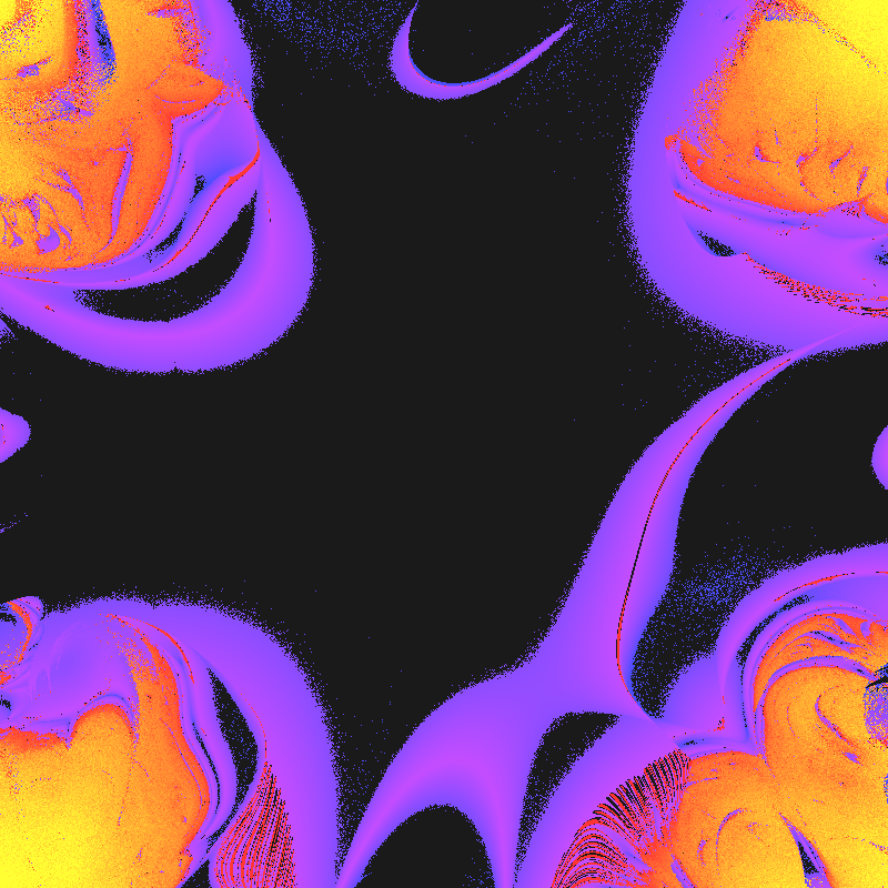
With a canvas size of 800 × 800, this image represents the properties of 640,000 different attractors. It also demonstrates that you can create compelling images not by drawing the attractors themselves, but by visualizing related metrics like exponents.

キャンバスサイズが800 x 800なので、640,000個のアトラクターの性質を調べて絵にしたものと言えます。これはアトラクターをそのまま描画するのではなく、関連する指数などを使っても面白い絵が作れるという例にもなっています。

The code is available on Codepen. Changing the values of $c$ and $d$ will reveal different images. Imagine a four-dimensional space with $a, b, c, d$ as its axes, densely packed with attractors. Since calculation takes time, we’re averaging 100 iterations after discarding the first 100 steps. To increase precision, try raising the value of calculationSteps.

コードはCodepenに置いてあります。 $c$ と $d$ の値を変えると違う絵が現れます。$a, b, c, d$ それぞれを軸にした4次元空間にアトラクターがびっしり詰まっているところを想像してみましょう。計算に時間がかかるので100回ステップを切り捨てた後の100回の平均をとっていますが、精度を上げたい場合は、calculationSteps の値を増やしてみましょう。

Equivalence of Lyapunov Exponent and KS Entropy

リアプノフ指数とKSエントロピーの等価性

When we introduced KS entropy, we didn’t explain the calculation in details. The method of dividing space into boxes and counting is difficult to implement in practice, depending on the system’s properties. But if you understand the Lyapunov exponent, you can use it as a shortcut to KS entropy.

KSエントロピーを紹介した時にその計算方法は詳しく説明しませんでした。空間を箱に分けて数えるという方法は実際に行おうとすると系の性質によってとても大変になるからです。ですが、リアプノフ指数の概念を知っているとそれをKSエントロピーへのショートカットとして使うことができます。

In chaotic systems, Pesin’s formula (Pesin’s Identity) connects the measure of how quickly trajectories diverge (Lyapunov exponent) with the measure of how quickly new information is generated (KS entropy).

カオス系において、軌道がどれくらいの速さで離れていくか（リアプノフ指数）という指標と、新しい情報がどれくらいの速さで生まれるか（KSエントロピー）という指標は、ペシンの公式（Pesin’s Identity）によって結ばれます。

$h_{KS} \approx \sum_{\lambda_i > 0} \lambda_i$

In multidimensional systems, space may stretch in multiple directions. The sum of all these stretching rates (positive $\lambda$) equals the rate of information generation. When two trajectories diverge, predicting where the next point will be becomes harder. Each time space stretches by a factor of 2 ($\lambda = \log_2 2 = 1$), we lose 1 bit of certainty about the system’s future—and the system generates 1 bit of new information. Think of it this way: when space doubles, we need an additional bit to record it with the same precision.

多次元のシステムでは、空間が引き伸ばされる方向が複数ある場合があります。そのすべての引き伸ばし率（正の $\lambda$）を合計したものが、そのまま情報の生成速度になります。2つの軌道が離れるということは、今の場所から「次がどこになるか」の予測がそれだけ難しくなるということです。空間が2倍に引き伸ばされる（$\lambda = \log_2 2 = 1$）ごとに、私たちはシステムの未来について 1ビット分 の確信を失い、同時にシステムは 1ビット分 の新しい情報を生成していると言い換えることができます。空間が2倍に引き延ばされると、その空間を同じ精度で記録するにはもう1ビット必要になると考えると良いでしょう。

If you’re wondering why it’s addition rather than multiplication in a multidimensional system, remember that the Lyapunov exponent is defined using logarithms.

多次元なのだから足し算じゃなくて掛け算じゃないかと思った人はリアプノフ指数が対数で定義されていることを思い出しましょう。

As we’ve seen, chaos doesn’t create new information from nothing. The information exists from the beginning—in the sense that the system is deterministic—but it’s hidden in digits too small for us to observe.

これまで見てきたように、カオスは新しい情報をゼロから作っているわけではありません。（決定論的である以上という意味で）情報は最初からそこに存在していますが、我々には観測できないほど微細な桁に隠されています。

Systems with positive Lyapunov exponents elevate information hidden in the microscopic universe, step by step, to higher-order digits. A state with positive KS entropy continuously translates the infinite information dormant in initial conditions into a visible macroscopic scale as time passes.

正のリアプノフ指数を持つ系は、このミクロな宇宙に隠された情報を、1ステップごとに上位の桁へと引き上げます。KSエントロピーが正である状態とは、初期値に眠っていた無限の情報を、時間の経過とともに目に見えるマクロなスケールへと絶えず翻訳し続けている状態なのです。

Topological Transitivity

位相的推移性

This property shows how thoroughly the system mixes. In a system with topological transitivity, trajectories starting from any region—no matter how small—will eventually reach every other region of the state space, given enough time. This is why chaos displays the same complexity wherever you look, and can be analyzed statistically as a random distribution.

これは、系がどれだけ強力にかき混ぜ（Mixing）を行っているかを示す性質です。位相的推移性がある系では、状態空間内のどのような小さな領域をとっても、そこから出発した軌道は、時間が経てば空間内の他のあらゆる領域へと入り込んでいきます。この性質があるからこそ、カオスはどこを切っても同じような複雑さを持っており、統計的にはランダムな分布として扱うことが可能になります。

Mathematically, a map $f: X \to X$ on a state space $X$ has topological transitivity when it satisfies this condition: for any two open sets $U$ and $V$ in the space (no matter how small) there exists a positive integer $n$ such that

数学的には状態空間 $X$ における写像 $f: X \to X$ が位相的推移性を持つとは、以下の条件を満たすことを指します。空間内の任意の2つの開集合（どんなに小さな領域でもよい）$U$ と $V$ に対して、ある正の整数 $n$ が存在し、

$f^n(U) \cap V \neq \emptyset$

This means that no matter which starting region ($U$) you choose, the points it contains will eventually appear within any other target region $V$ if you wait long enough. If trajectories from a certain region can never reach some isolated area, the system is not transitive. In chaos, the entire space must form a single connected vessel.

要はどんな出発点（領域 $U$）を選んだとしても、そこに含まれる点は、十分な時間をかければターゲットとした別の領域 $V$ の中にいつか現れるということです。もし、ある領域から出発した軌道が一生たどり着けない孤立した領域があるなら、その系は推移的ではありません。カオスにおいては、空間全体が1つながりの器になっている必要があります。

Topological transitivity doesn’t guarantee that the system fills the entire space—for example, every possible $x, y$ value in two dimensions. Instead, it means that within the structure the system traces, all regions are connected as one. From anywhere within that structure, you can reach anywhere else. This sounds almost tautological but no matter how much time passes, trajectories will never enter regions outside the system’s reach or holes within the structure where trajectories don’t pass.

位相的推移性が保証するのは、空間全体（例えば2次元であればあらゆる $x, y$ の値）を埋め尽くすことではありません。あくまで、その系が描く構造の内部において、あらゆる領域が1つつながりになっており、その中のどこからでも他のどこへでも到達できる、という性質を指しています。ほとんどトートロジーですが、系が到達できる範囲の外側や構造の中に存在する穴（軌道が通らない場所）には、どれだけ時間をかけても入り込むことはありません。

Density of Periodic Orbits

周期的軌道の稠密性

A map $f: X \to X$ on a state space $X$ has dense periodic orbits when it satisfies the following condition:

状態空間 $X$ における写像 $f: X \to X$ が周期軌道の稠密性を持つとは、以下の条件を満たすことを指します。

For any point $x$ in $X$ and for any arbitrarily small real number $\epsilon > 0$, there exists a periodic point $p \in X$ such that $d(x, p) < \epsilon$.
$X$ 内の任意の点 $x$ と、どんなに小さな実数 $\epsilon > 0$ に対しても、ある周期点 $p \in X$ が存在し、$d(x, p) < \epsilon$ である。

Here, $d(x, p)$ is the distance between $x$ and $p$, and a periodic point $p$ is a point for which there exists some positive integer $k$ such that $f^k(p) = p$.

ここで $d(x, p)$ は $x$ と $p$ の間の距離、周期点 $p$ とは、ある正の整数 $k$ に対して $f^k(p) = p$ となる点のことです。

This is challenging to grasp, but it means that no matter which point $x$ you choose in the system, there’s an orbit hiding right nearby within a distance of $\epsilon$ that starts from a point (p) and returns to itself ($f^k(p) = p$).

わかりにくいですが、これは系の中のどんな点 $x$ を選んでもそのすぐそば、距離 $\epsilon$ の内側にその点（p）からスタートして元の点に戻ってくる（$f^k(p) = p$）軌道が隠れている、という主張です。

$f^k$ is the function that advances time to find the next position, corresponding to one step in the logistic map or Clifford attractor. For continuous systems, we consider the operator $\phi_t(x)$ that advances the state by time $t$, but the rest of the content is the same.

$f^k$ は時間を進めて次の位置を求める関数、ロジスティック写像やクリフォードアトラクターの1ステップに相当します。連続系では時間 $t$ だけ状態を進める演算子 $\phi_t(x)$ を考えますが、残りの内容は同じです。

In mathematics, “dense” means existing closely packed without gaps. Just as you can find a rational number arbitrarily close to any point on the real number line, periodic orbits are woven throughout chaos like a mesh network. The definition’s $d(x, p) < \epsilon$ shows that a periodic point $p$ exists arbitrarily close to any state $x$—but this doesn’t mean $x$ itself lies on a periodic orbit. This is similar to how rational numbers are dense, yet infinitely many irrational numbers are packed between them.

数学において稠密（ちゅうみつ）とは、隙間なくびっしり存在することを指します。例えば、実数直線のどこを切ってもそのすぐ傍に有理数が見つかるように、カオスの中には規則正しい周期軌道が網の目のように張り巡らされています。定義にある $d(x, p) < \epsilon$ は、状態 $x$ のどんなに近くにも周期点 $p$ があることを示していますが、$x$ そのものが周期軌道上にあるとは限りません。これは、有理数が稠密であっても、その間には無限個の無理数が埋まっていることと似ています。

Most points in chaos, like these irrational numbers, are slightly displaced from periodic orbits and are therefore destined never to return to their starting position.

カオスにおけるほとんどの点は、この無理数のように周期軌道からわずかにずれた位置にいるため、決して元に戻らない運命にあります。

Imagine chaos not as independent random motion, but as a collection of infinitely many unstable periodic orbits. A particle tries to follow a certain periodic orbit $A$, but gets ejected due to a slight deviation. It then gets caught by a neighboring periodic orbit $B$, is ejected again, and repeats this process infinitely. This dynamics of eternally jumping between infinite periodicities is the true nature of chaos’s character: maintaining a certain form (the attractor) despite never passing through the same place twice.

イメージとしては、カオスとは独立したデタラメな動きではなく、無限にある不安定な周期軌道の集合体です。粒子はある周期軌道 $A$ に添おうとしますが、わずかなずれによって弾き出されます。すると次に、隣り合う周期軌道 $B$ に捕まり、また弾き出され、というプロセスを無限に繰り返します。この無限の周期性の間を永遠に飛び移り続ける動態こそが、二度と同じ場所を通らないにもかかわらず、一定の様式（アトラクター）を維持し続けるという、カオスの姿の正体なのです。

Ergodicity

エルゴード性

Though not part of the formal definition of chaos, ergodicity is an important related concept.

カオスの条件には含まれませんが、関連した重要な概念としてエルゴード性があります。

While the three conditions of chaos focus on the topological structure of mixing, ergodicity concerns the statistical property of how time is distributed across different locations.

カオスの3条件がどのように混ざり合うかという位相的な構造に注目するのに対し、エルゴード性はある場所にどれだけの時間滞在するかという統計的な性質を問題にします。

A system has ergodicity when its time average and space average coincide. Think of the time average as tracking a single trajectory from a starting point and observing how it fills the space. The space average, in contrast, shows how tens of thousands of points are distributed across space at a single moment in time.

ある系にエルゴード性があるとは、その系の時間平均と空間平均が一致するという意味です。ここで、時間平均とはある点からスタートする軌跡を追い続けて、その軌跡がどのように空間を塗りつぶすか、空間平均とはある瞬間に何万個もの点をバラまいた時に空間上にどのように散らばるかだと考えると良いでしょう。

$\lim_{n \to \infty} \frac{1}{n} \sum_{i=0}^{n-1} \phi(f^i(x)) = \int_X \phi(x) , d\mu(x)$

The left side of this equation is the time average, obtained by tracking a single trajectory and averaging it.

• $x$: Starting point.
• $f^i(x)$: Position after $i$ steps.
• $\phi(x)$: Measure function. Returns whatever value you want to measure at that location (for example, distance from the origin, or a flag indicating whether the point is within a specific pixel).
• $\frac{1}{n} \sum$: The average value obtained by dividing the sum of values obtained over $n$ steps by the number of steps. Since it’s $\lim_{n \to \infty}$, theoretically this is repeated infinitely.

この数の左辺が時間平均で、1つの軌跡を追いかけて平均値したものです。

• $x$：スタート地点。
• $f^i(x)$：$i$ ステップ後の位置。
• $\phi(x)$：測度関数。入力に対して何らのその場で測りたい値を返す（例えば、原点からの距離や、あるいはその点が特定のピクセル内にあるかというフラグ）。
• $\frac{1}{n} \sum$：$n$ 回のステップで得られた値の合計を回数で割った平均値。 $\lim_{n \to \infty}$ なので理論上は無限回繰り返される。

The right side is the average value of everyone scattered throughout the entire space at a given moment.

• $X$: All regions where the system can exist (the entire attractor).
• $\mu$: A measure representing the weight of each location (invariant measure).
• $\int_X \dots d\mu$: Measuring values at every location on the attractor, multiplying by the “weight” of each location, and summing them up.

右辺はある瞬間に空間全体にばら撒かれた全員の平均値です。

• $X$：系が存在できるすべての領域（アトラクター全体）。
• $\mu$：その場所の重みを表す尺度（不変測度）。
• $\int_X \dots d\mu$：アトラクター上のあらゆる場所で値を測定し、それぞれの場所の「重み」を掛け合わせて足し合わせたもの。

When interpreting this equation, note a few key points. First, the measure function $\phi(x)$ can be any arbitrary function. Since this equation focuses on whether the results match, any function that produces different results for different trajectories will work. Second, regarding $\mu$, it seems the equation can always hold simply by choosing weights to match the left side.

この式を解釈する上で注意すべき点がいくつかあります。まず測度関数 $\phi(x)$ は任意の関数ですがこの式は結果が同じになるかという点に注目しているので、乱暴に言うと異なる軌跡に対して異なる結果が出るものであればなんでも構いません。次に $\mu$ ですが、これは左辺の結果に合うように重みを選べばいいだけなので実は確実に式を成立させてしまうように見えます。

The key point is that a unique invariant measure $\mu$ exists such that the time average matches the space average, regardless of which $x$ you randomly choose on the left side. This means the system is unified—wherever you select a starting point, you’re guaranteed to pick one that represents the entire system. This property is stronger than topological transitivity. While topological transitivity only ensures all points can be reached, ergodicity guarantees that the density of time spent at different locations is also the same.

大事なのは左辺でランダムに $x$ を選んでも時間平均が空間平均に一致する唯一の不変測度 $\mu$ が存在すると言うことで、これは系が分断されておらず、どこを選んでもその系を代表する点を選ぶことが保証されていると言うことです。これが位相的推移性より強いのは、位相的推移性が全ての点にたどり着くと主張しているだけなのに対して、エルゴード性は滞在の仕方の濃淡まで同じだと言っていることです。

This is a very subtle point, but saying “regardless of which $x$ you randomly choose” does not mean it holds for all points. Consider the probability of randomly dropping a needle on a number line and hitting exactly a rational number. Rational numbers exist infinitely and densely everywhere, but compared to the overwhelming volume of irrational numbers filling the gaps between them, their size (measure) is mathematically zero. Similarly, chaos contains countless hidden special points where it doesn’t hold, but since they have no area, the probability that a randomly chosen initial value falls into that trap is zero.

これは非常に微妙な点なのですが、「ランダムに $x$ を選んでも」と言うのは、全ての点で成立するという意味ではありません。数直線の上にランダムに針を落として「有理数」にぴたりと当たる確率を考えてみてください。有理数は無限に、しかも至る所に（稠密に）存在しますが、その隙間を埋める無理数の圧倒的なボリュームに比べれば、その大きさ（測度）は数学的にゼロです。同様に、カオスの中にも成立しない特殊な点は無数に隠れていますが、それらは面積を持たないため、適当に選んだ初期値がその罠に落ちる確率はゼロなのです。

Though it sounds complicated, in simple terms: among chaotic systems, those with ergodicity will produce the same overall pattern regardless of the initial starting point.

ゴチャゴチャと難しいようですが大雑把に言うとこれは、カオスの中でもエルゴード性があるものは初期値が違っても同じ絵に落ち着くよ、と言うことを言っています。

The Clifford attractor generally has ergodicity depending on parameter settings, so let’s test it. In the code below, we start from two different points and draw each trajectory in red and blue. The result appears as a single purple color rather than two distinct colors, showing that these two trajectories match almost perfectly.

クリフォードアトラクターはパラメーター設定によりますが大体エルゴード性を持つので、テストしてみましょう。下のコードでは2つの異なる点からスタートして赤と青でそれぞれの軌跡を描きます。結果が2色ではなく紫一色に見えるのはこの2つの軌跡の結果がほぼ完全に一致していることを示します。

Do they apply to the real world?

現実世界にも当てはまるのか

Chaos theory has its origin in efforts to understand complex real-world phenomena like weather. But like all theories, it has limitations when applied to reality that we need to recognize.

カオス理論は気象のような現実世界の複雑な現象を理解することに起源を持っていますが、他のすべての理論と同様に、現実に適用する際にはその限界を知る必要があります。

For example, simple models like the Lorenz attractor strictly guarantee topological transitivity. But we cannot just apply this property to Earth’s weather. While the theoretical model may satisfy transitivity, it’s impossible to strictly define the weather system and confine it within a closed box. Think about fluctuations in solar activity, volcanic eruptions, human activities. Are these outside the system or inside it?

例えば、ローレンツ・アトラクターのようなシンプルなモデルでは、位相的推移性は厳密に保証されます。しかし地球の気象を考える場合、理論モデルはこの性質を満たすかもしれませんが、現実にはこの推移性を安易に適用できません。なぜなら、気象という系を厳密に定義し、閉じた箱の中に閉じ込めることは不可能だからです。太陽活動の変動、火山の噴火、人間の活動などについて考えて見ましょう。これらは系の外でしょうか、それとも中でしょうか。

Nevertheless, when we define a specific scope, theoretical models can approximate reality well enough to provide valuable insights. They become fascinating subjects worthy of study. But since chaos has an inherent property that slight differences in input produce completely different results, models capable of accurately predicting the future are fundamentally impossible.

それでも理論モデルは、特定の視野に絞れば、現実を十分に近似し、素晴らしい洞察を与えてくれます。研究に値する非常に面白い素材となり得るのです。一方でカオスは、その性質上、わずかな入力の違いで全く異なる結果を生むため、未来を正確に予測するモデルは原理的に不可能だと言えるでしょう。

To Learn More

より学ぶために

So far, we’ve explored various examples and theories related to chaos. Let’s think about whether you can develop these into your own unique expressions.

ここまでカオスに関する様々な例や理論を見てきました。これらを参考に独自の表現に発展させられるか考えてみましょう。

In Folds, you can find examples of drawing various beautiful patterns with discrete steps similar to the Clifford attractor.

Foldsでは、クリフォードアトラクターに似た離散的なステップで様々な美しいパターンを描く例が見られます。

When working with chaotic elements in graphics, existing systems like the Lorenz attractor are sometimes used as convenient number generators. But more often, the goal is simply to achieve a chaotic texture or behavior—whether the system is strictly chaotic doesn’t really matter. For example, can you bring out characteristics like initially aligned trajectories diverging exponentially over time while using random inputs or noise? Think about how you can apply the concepts learned here to your own visual ideas.

グラフィックスなどでカオス的なものを扱う時には既存のシステム、例えばローレンツアトラクターなどをいい感じの数値の発生器として使うこともありますが、それよりもカオス的な質感や振る舞いを得ることが目的で、系が厳密にカオスかどうかはどうでも良いことの方が多いでしょう。例えばランダムな入力やノイズを用いつつもカオス的な見た目、例えば最初は揃っていた軌道が時間と共に指数関数的にずれていく、といった特徴をうまく出すことはできるでしょうか。ここで学んだ概念をビジュアルな発想に落とせるか考えてみましょう。

To learn more about the theory, search or ask AI using keywords from this page. You might also explore fractal dimensions, which measure the complexity of shapes created by chaos. See the Fractal フラクタル page as well as a reference.

もしより理論について学びたければこのページに登場するキーワードをもとに検索したりAIに聞いてみたりすると良いでしょう。カオスが作る形のスカスカ具合を数値化するフラクタル次元について調べて見るのも面白いと思います。Fractal フラクタル のページも参照してください。